If you’ve ever had a formula like =A1=B1 return FALSE—even though the values in A1 and B1 seem exactly the same—you’ve run into one of Excel’s most puzzling quirks: the floating-point error. These tiny differences are usually invisible, but they can cause formula checks and even conditional formatting rules to fail in unexpected ways. This article explains why these errors happen, how to spot them, and how to fix them with simple techniques like rounding.
- Why Your Numbers Don’t Add Up
- What Is a Floating Point Error?
- Example 1 - Typical rounding problem
- Example 2 - Floating point errors with subtraction
- Example 3 - Floating point errors with incremental addition
- Set precision as displayed (not recommended)
- Other rounding functions in Excel
- Takeaways
- Floating point details
- Useful Links
Why Your Numbers Don’t Add Up
When working with numbers in Excel, especially when adding or subtracting many values during reconciliation, you may run into small discrepancies that seem illogical, like two totals that should match but don’t. There are two basic reasons why you might run into this situation:
- A simple rounding problem.
- A floating-point error.
The first problem is more common and is often related to Excel’s number formatting or sometimes to the column width. The second problem is less common and more difficult to understand. It happens because Excel uses binary floating-point numbers, which can’t represent some decimal values exactly. As a result, tiny rounding errors accumulate during calculations, creating results that are extremely close but not exactly equal. These differences are often invisible on the worksheet but can cause equality checks or balance comparisons to fail unexpectedly:
- A conditional formatting rule shows a calculated number in red when it should be green.
- A formula that checks a calculation unexpectedly returns FALSE.
- A final balance does not equal the expected result, although it appears to be correct.
This problem is not limited to Excel. Other environments and computer languages have the same limitation.
What Is a Floating Point Error?
Excel uses the decimal number system to display results. This is the base-10 system we use every day, with ten digits (0 through 9) to represent all numbers. In decimal, each digit’s position in a number represents a power of 10, with values increasing from right to left. Computers, however, (including Excel) store numbers using a system called floating-point arithmetic, based on binary (base 2). In binary, only two digits (0 and 1) are used, and each position represents a power of 2. This system is efficient for computation, but it has an important limitation: many decimal values can’t be represented exactly in binary.
For example, numbers like 0.1 and 0.2 can’t be represented perfectly in binary, so Excel stores values like 0.10000000000000001 and 0.20000000000000001 instead. Likewise, 1/3 doesn’t have an exact decimal representation (it becomes 0.3333333…). As a result, when Excel stores these values, it must approximate them. These tiny approximations—called floating-point errors—can cause surprising results when performing calculations or comparisons
Let’s look at some examples, starting with a problem that is not a floating-point error.
Example 1 - Typical rounding problem
Before we get into specific examples of floating-point errors, let’s look at a typical rounding problem. This is not a floating-point error, but rather a misunderstanding created by the way that Excel displays numbers when number formatting is applied. In the worksheet below, we have a list of products in column B and corresponding prices in column C. In column D, we have calculated a 10% discount with a formula like this:
=C5*10%

In column F, we have manually entered the same discount. In column G, we have a formula that checks the calculated discount in column C against the hardcoded discount in column F. The formula in G5 is:
=D5=F5

In all rows, it returns FALSE. What’s going on?
The problem is that the calculated values in column D are not rounded, but they look rounded because a Number format with 2 decimal places has been applied to them. Number formats in Excel change the way a number is displayed, but they do not change the underlying number. If we change that number format to show four decimal places, you can see the problem clearly:

Tip: Another way to see more decimal places, temporarily apply the General number format with the shortcut Ctrl + Shift + ~. Depending on the number, Excel will display up to 9 decimal places if the column is wide enough. Then Ctrl + Z to undo.
The discounts in column D are not rounded, but the number format with 2 decimal places causes them to look rounded. On the other hand, the numbers typed into column F are actually rounded to two decimal places. This is why none of the numbers match. If you need to compare these numbers apples-to-apples in a case like this, a good option is to modify the check formula in G5 like this
=ROUND(D5,2)=F5
This formula uses the ROUND function to round the value in D5 to two decimal places before comparing it to the value in F5. The advantage of this approach is that it leaves the original values in column D unchanged, but still lets you compare to the expected results. With this change, you can see that now the check formula in column E returns TRUE in all rows:

Another option is to round the values in column D right from the start using a formula like this in D5:
=ROUND(C5*10%,2)
This option will actually round the discounts in column D to two decimal places, and they will match the hardcoded values in column F. Both options are valid, but I would generally avoid rounding the discounts unless you have a reason to do so.
To summarize, this is a rounding problem, not a floating-point error. Number formats in Excel can make it appear as though numbers are the same even when they aren’t.
Tip: Avoid rounding too early in your calculations, unless it is required. Early rounding can introduce cumulative errors. Instead, calculate precisely first, then apply rounding only at the final step. This method preserves accuracy.
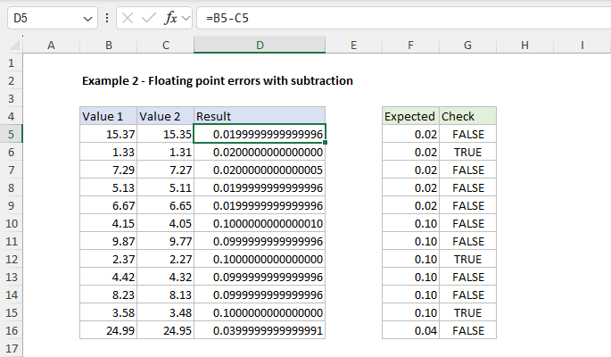
Example 2 - Floating point errors with subtraction
Now let’s look at an example of actual floating-point errors. In the worksheet below, we are subtracting numbers in column C from the numbers in column B. The formula in D5 looks like this:
=B5-C5

The values in columns B and C are ordinary numbers with exactly two decimal places, like dollars and cents. Column D contains the calculated result, and column E contains the expected result (hard-coded). If you look at the numbers in columns B and C, you can probably guess what the result should be. The formula in column F compares the actual result to the expected result, like this:
=D5=E5
As you can see, most of the checks in column G are FALSE, even though we would expect all results to be TRUE. This is quite confusing. The calculation is simple, and the results look perfectly ordinary. What’s going on here? This is a case where some of the numbers in column D can’t be perfectly stored as binary numbers. They look normal, but if we look more carefully, we can find some tiny problems.
The first thing to check is the raw numbers. To show more decimal places, use the keyboard shortcut Ctrl + 1 to open the Format cells dialog box, then navigate to Number and set the decimal places to 16:

Then adjust the column width to show the full value. Now we can see that some of these numbers are not what they appear to be:
Tip: Another way to increase decimal places is to punch the “increase decimal” button on the ribbon 16 times, but I like the Ctrl + 1 method because it’s fast and you can quickly undo with Ctrl+Z after checking the raw number. Note also if you want to check a static number typed or pasted into Excel, the formula bar will show the number in its raw form without number formatting.
Now that we know the problem, how should we fix it? One way to fix a floating-point error in Excel is to add rounding to the appropriate formulas. For example, in this worksheet, we can modify the Check formula to round the value in column D5 before testing. Since we’re working with numbers that are accurate to two decimal places, we can use the ROUND function with num_digits set to 2. You can see this approach in the worksheet below, where the formula in G5 is now:
=ROUND(D5,2)=F5

Another good way to manage floating-point errors is to use a formula that ensures that calculated and expected results are within a specified tolerance. We can use the ABS function to create a tolerance-based check like this:
=ABS(D5-F5)<0.0000000001
We first subtract the expected result from the calculated result. Then we take the absolute value, and check the difference is less than 0.0000000001. This method allows you to bypass rounding entirely, by defining a threshold for how close is “close enough.” You can see this formula in action below:

Note: The tolerance above is very small. In general, you should adjust the tolerance to suit the specific use case.
Example 3 - Floating point errors with incremental addition
Floating-point errors can also appear when you add the same decimal value repeatedly. In the worksheet below, we are repeatedly adding 0.1 to a starting value of -1.9. All values in column B are generated with the SEQUENCE function with this formula in cell B5:
=SEQUENCE(F6,,F4,F5)
We would expect to reach 1 in row 14 after adding 0.1 nine times. However, for some reason, the value in cell B14 is not exactly 1. The values in column C are expected results. The yellow highlighting indicates rows where the calculated value does not equal the expected value. What is going on here?

In the screen below, we have formatted values in column B to display 15 decimal places, then expanded the column as needed. Now we can see the source of the problem clearly:

All values in the range B14:B24 are very slightly different from expected because of floating-point errors. These errors show up here because Excel internally can’t represent increments of 0.1 in binary exactly. As we incrementally add 0.1, the small errors accumulate, resulting in values like -0.999999999999999 instead of -1.0.
To eliminate this problem, we can simply round each result to a suitable number of decimal places. In this case, the intent is clearly to work at 1 decimal place precision. So we should use around to 1 decimal place. This is actually the formula used in column C to calculate expected values:
=ROUND(SEQUENCE(F6,,F4,F5),1)

The original SEQUENCE formula above is now nested inside the ROUND function as the number argument, with 1 for num_digits . The results in column C are now cleanly incremented in steps of 0.1. To compare the original raw values with the rounded values, we use a conditional formatting rule applied with this formula:
=$C5<>$B5
This highlights the rows where the rounded values are different from the raw values. In other words, the yellow highlight shows where floating-point errors have created an unexpected result.
Tip: Round to match your intended precision. For step sizes of 0.1, use 1 decimal place. For cents, use 2. Don’t round too early—round late in the process or at the point of comparison.
Set precision as displayed (not recommended)
There is another way to fix problems related to floating-point errors, using an Excel setting called “Set Precision as Displayed.” This is a dangerous setting that essentially truncates any part of a number that isn’t visible on screen. In other words, “what you see is what you get.” While this is a very fast way to change hundreds or thousands of numbers, it should be used with extreme caution. This option forces Excel to store numbers exactly as they are displayed on screen by permanently altering the stored precision of numbers, which can result in permanent data loss. Also, because the setting applies globally across the workbook, it can impact unrelated calculations on different worksheets. As a result, I do not recommend this approach unless you fully understand its implications and are certain it won’t negatively impact other data.
Other rounding functions in Excel
Although the ROUND function is fine for the purposes shown above, Excel has a whole group of rounding functions you can use to fix floating-point problems and rounding problems in general:
- ROUND : Round to a specific number of digits
- ROUNDUP : Always rounds up, away from zero
- ROUNDDOWN : Always rounds down, toward zero
- MROUND : Rounds to the nearest multiple
- CEILING : Rounds up to the nearest multiple
- FLOOR : Rounds down to the nearest multiple
- INT : Rounds down to the nearest integer
- TRUNC : Removes the decimal part without rounding
Key Takeaways
- Floating-point errors in Excel are due to Excel’s internal representation of numbers using floating-point arithmetic. They can happen at any time, but they don’t normally cause problems because they involve tiny values.
- If you are comparing calculated results with expected results directly, you can run into floating-point errors in a way that is surprising and confusing. In general, values that seem identical will be flagged as different.
- These issues can be easily managed by being aware of the possibility and understanding why they happen.
- One way to fix the problem is to round strategically, typically late in your calculations or inside the formula that checks results.
- Another good option is to switch to a formula that confirms numbers are within a given tolerance. This approach involves no rounding and maintains maximum precision.
- A final option to resolve floating-point errors is to use Excel’s “Set precision as displayed” feature to force Excel to store numbers as displayed. You shouldn’t use this option unless you fully understand the implications.
Floating point details
Excel performs floating-point math according to the IEEE 754 standard, which is the foundation for how decimal numbers are stored and calculated in nearly all modern software.
When you type a number or use the = operator in Excel, the value is limited to 15 significant digits—the maximum precision Excel stores. If the digits match, Excel considers the numbers equal, even if tiny differences exist beyond that point. For example, both 0.1 + 0.2 and a hardcoded 0.3 round to the same stored value, so =0.1 + 0.2 = 0.3 returns TRUE.
In theory, subtracting the same values like this: =(0.1 + 0.2) - 0.3 should expose a small error like 5.55E-17, because these decimal values can’t be stored exactly in binary. But in current versions of Excel, the result is often 0.
This is because Excel appears to have a “feature” that “zeroes out” very small results in certain arithmetic operations. The exact behavior isn’t documented by Microsoft (as far as I know), but it helps avoid distracting floating-point glitches in many common cases.
Even with this safeguard, floating-point errors can still appear in other ways, especially with larger calculations, comparisons, or repeated operations. The best solution remains the same: use rounding when precision matters.
Useful Links
Floating-point arithmetic may give inaccurate results in Excel (Microsoft)
Numeric precision in Microsoft Excel (Wikipedia)
Floating point explanation desired (reddit)
What is regex?
A brief history of regex in Excel
Regex vs. Excel wildcards
Why regex is useful in Excel
The REGEXTEST function
The REGEXEXTRACT function
The REGEXREPLACE function
Regex quick reference
Important regex terminology
Regex anchors
Regex tips
Summary
What is regex?
What is regex? Regex, short for Regular Expressions, is a powerful tool for pattern matching in text data. Using a combination of metacharacters, literal characters, character classes, and quantifiers, you can define complex search patterns to extract, validate, or manipulate text data. See examples below . The main benefit of regex in Excel is the ability to work with text very precisely without resorting to complicated formulas that are hard to understand and maintain. In Excel, Regex support comes primarily from the introduction of three brand-new functions:
- The REGEXTEST function
- The REGEXREPLACE function
- The REGEXEXTRACT function
In addition to the three dedicated functions above, XLOOKUP and XMATCH have also been upgraded to support regex. Plus, you can use the functions above inside other formulas to instantly upgrade their capabilities. For example, you can use REGEXTEST inside the IF function as the logical test, which “upgrades” IF to support regex. In this article, I’ll introduce Excel’s new regex functions and provide examples of how these functions are helpful. But first, let’s review how we got here.
Many existing guides to using Regular Expressions in Excel on the web are based on VBA or custom add-ins. However, in Excel 365, you don’t need to use VBA or add-ins to use Regular Expressions because regex support is built-in. This guide covers the native regex support added to Excel via the three regex functions listed above.
A brief history of regex in Excel
Why doesn’t Excel support Regex? This is one of those questions that has bothered Excel power users for many years. It’s been a topic of heated debates and the cause of many clunky, complicated formulas. Although regex is a standard feature in many programming languages, it was notably absent from Excel for most of its history. Here’s how Excel’s text processing capabilities evolved:
- Excel has always supported basic wildcards (* and ?), but these are primitive compared to regex patterns. Users had to rely on combining functions like LEFT, RIGHT, MID, FIND, SEARCH, and SUBSTITUTE for pattern matching, resulting in complex, hard-to-maintain formulas.
- Power users worked around these limitations using VBA, Power Query, or custom add-ins for regex support, but these tools require different skills and are not available to all users.
- In Excel 2013, Microsoft added some regex-like capability with the FILTERXML function, which uses XPath queries for pattern matching. Still, this function is not widely used or available in Excel for Mac.
- In 2022, Microsoft improved text handling with TEXTSPLIT, TEXTBEFORE, and TEXTAFTER functions. These functions make it much easier to split text at specific locations in an Excel formula. However, they do not support regex.
- In December 2024, Excel introduced three regex functions: REGEXTEST, REGEXREPLACE, and REGEXEXTRACT. These functions modernize Excel’s text-processing capabilities and bring it up to speed with other professional tools.
Now that Excel supports regex directly, many complicated formulas of the past can be drastically simplified.
Regex vs. Excel wildcards
Excel wildcards are like a toolbox with just two tools: * for “anything” and ? for “one thing.” Sure, you can find “apple*” or “?at,” but that’s about it. They’re the flip phone of pattern matching.
Regex is a different story. While wildcards are asking “Does this have an “a” followed by… stuff?”, regex is performing complex queries like “Any word that starts with a capital letter, contains exactly two numbers, and ends with x or y but not z”.
Want to match exactly three digits followed by optional whitespace and a hyphen? Try \d{3}\s*- Need to find an email address or validate a strong password? Regex has patterns for that. It can even “look ahead” in your text to match patterns only when they occur before something else.
You get the idea. Regex goes far beyond basic wildcards.
Why regex is useful in Excel
Before we get into the details, let’s look at a specific example of how regex can help simplify a formula. In the workbook below, the goal is to extract the numbers from the product codes in column B. With hundreds of functions available, you might think this is a simple problem in Excel, but it’s not! The problem is that the numbers vary in length, and their location in the product code also changes. There’s just no easy way to figure out where each number begins and ends. Instead, the formula below in cell D5 takes a “brute force” approach and simply removes all non-numeric characters. It looks like this:
=TEXTJOIN("",TRUE,IFERROR(MID(B5,SEQUENCE(LEN(B5)),1)+0,""))

It’s not exactly obvious what this formula is doing, right? You can find an explanation here . It’s pretty complicated, and I’m even cheating a bit because I’m assuming at least Excel 2021, which has the SEQUENCE function . In Excel 2019, things get uglier because we need to spin up our own number array with the volatile INDIRECT function and the ROW function:
=TEXTJOIN("",TRUE,IFERROR(MID(B5,ROW(INDIRECT("1:"&LEN(B5))),1)+0,""))
In Excel versions before 2019, the formula becomes even more complicated!
What about regex? Does it help in this case? Yes . Regex helps a lot! In the worksheet below, the new formula in cell D5 is based on the REGEXEXTRACT function. Here it is:
=REGEXEXTRACT(B5,"\d+")
Yep, that’s the whole formula. Basically, we are asking REGEXEXTRACT for a sequence of 1 or more numbers. You can see the results below. I think you’ll agree that this new formula is a lot simpler 🙂

Now that you have a taste of how regex can help simplify difficult formulas, let’s look more closely at the three new regex functions.
The REGEXTEST function
The Excel REGEXTEST function tests for a given regex pattern. The result from REGEXTEST is TRUE or FALSE. For example, =REGEXTEST(A1,"[0-9]") will return TRUE if cell A1 contains any numeric digit, and =REGEXTEST(A1,"[A-Z]") will return TRUE if A1 contains any uppercase letters. REGEXTEST opens up new possibilities for data validation and text analysis directly within Excel formulas. In the worksheet below, REGEXTEST is configured to test addresses for one of four US states: MN, MT, ND, and SD. The formula in D5, copied down, looks like this:
=REGEXTEST(B5,"\b(MN|MT|ND|SD)\b")
The pattern “\b(MN|MT|ND|SD)\b” matches MN, MT, ND, or SD. The ‘\b’ is a word boundary character. It will match a space and any punctuation that typically appears around a word. The ‘|’ creates OR logic.

Note: While you probably don’t need a TRUE or FALSE result in a case like this, you could use exactly the same formula above inside the FILTER function to list all addresses that contain MN, MT, ND, or SD.
The REGEXEXTRACT function
The REGEXEXTRACT function extracts specific information from a string based on a Regex pattern. It’s perfect for pulling out key pieces of data from messy text. For example, in the worksheet below, the goal is to extract telephone numbers in the format xxx-xxx-xxxx from the text strings in column B. The formula in cell D5, copied down, looks like this:
=REGEXEXTRACT(B5,"\d{3}-\d{3}-\d{4}")

This example gives you a sense of regex’s power and flexibility. This formula is looking for and extracting phone numbers that follow a pattern like this: “123-456-7890”. Let’s break down each part:
- ‘\d{3}’ looks for exactly 3 digits
- ‘-’ looks for a hyphen
- ‘\d{3}’ looks for 3 more digits
- ‘-’ looks for another hyphen
- ‘\d{4}’ looks for 4 more digits
So, if you have text that contains something like “My phone number is 555-123-4567”, this formula will pull out just “555-123-4567”.
The REGEXREPLACE function
The REGEXREPLACE function allows you to replace parts of a string that match a regex pattern with something else. It’s very useful for cleaning up or reformatting text. You can think of REGEXREPLACE as a much more powerful version of the simplistic SUBSTITUTE function . For example, in the workbook below, REGEXREPLACE is configured to remove all non-numeric characters from the telephone numbers in column B. The formula in cell D5, copied down, is:
=REGEXREPLACE(B5,"[^0-9]","")

The pattern “[^0-9]” will match any character that is not a number. Since the replacement pattern is an empty string (""), the result is that REGEXREPLACE effectively “strips” all non-numeric characters from the input, and the final result contains numbers only.
Regex quick reference
Regex relies on patterns to match specific text. The table below contains some simple regex patterns. These patterns can be combined to create very capable text-matching formulas.
| Pattern | Description and examples |
|---|---|
| abc | Matches the literal text ‘abc’. Example: ‘abc’ matches ‘abc’, but not ‘ABC’ or ‘ab’. |
| . | Matches any single character except a newline. Example: ‘c.t’ matches ‘cat’, ‘cot’, ‘c@t’. |
| \d | Matches any digit (0-9). Example: ‘\d\d\d’ matches ‘123’, ‘999’. |
| \w | Matches any word character (letter, digit, underscore). Example: ‘\w\w’ matches ‘ab’, ‘1_’, ‘A9’. |
| \s | Matches any whitespace character (space, tab, newline). Example: ‘a\sb’ matches ‘a b’. |
| \b | Matches a word boundary. Example: ‘\bcat\b’ matches ‘cat’ in ’the cat sits’ but not ‘category’. |
| [abc] | Matches any one character listed in brackets. Example: ‘gr[ae]y’ matches ‘gray’ and ‘grey’. |
| [a-z] | Matches any one character in the range. Example: ‘[a-z]’ matches any lowercase letter. |
| [^abc] | Matches any character NOT listed. Example: ‘[^0-9]’ matches any non-digit. |
| a* | Matches 0 or more ‘a’. Example: ‘ca*t’ matches ‘ct’, ‘cat’, ‘caaat’. |
| a+ | Matches 1 or more ‘a’. Example: ‘ca+t’ matches ‘cat’, ‘caat’, but not ‘ct’. |
| a? | Matches 0 or 1 ‘a’. Example: ‘colou?r’ matches ‘color’ and ‘colour’. |
| a{3} | Matches exactly 3 ‘a’. Example: ‘a{3}’ matches ‘aaa’, but not ‘aa’ or ‘aaaa’. |
| a{2,4} | Matches 2 to 4 ‘a’. Example: ‘a{2,4}’ matches ‘aa’, ‘aaa’, ‘aaaa’. |
| ^abc | Matches ‘abc’ at start of string. Example: ‘^The’ matches ‘The cat’ but not ‘In The’. |
| abc$ | Matches ‘abc’ at end of string. Example: ‘.com$’ matches ’example.com’. |
| (abc) | Groups pattern and captures match. Example: ‘(cat|dog)s’ matches ‘cats’ and ‘dogs’. |
| (?:abc) | Non-capturing group. Like () but doesn’t store the match. |
| a|b | Matches ‘a’ or ‘b’. Example: ‘cat|dog’ matches ‘cat’ or ‘dog’. |
Regex terminology
Because Regex is essentially a mini-language, it has its own vocabulary. Here is a list of some important terminology:
- Pattern - The actual sequence of characters that defines the regex. For example \d+ is a pattern for one or more digits.
- Literal - Characters in a regex pattern that match themselves. For example, in cat , the literals are c , a , and t .
- Metacharacter - Characters with special meanings in regex. For example, a period . matches any character, ^ matches the start of a string, $ matches the end of a string.
- Character Class - A set of characters enclosed in square brackets [] that matches any one of the characters inside. For example, [aeiou] matches any vowel.
- Quantifier - Specifies how many instances of a character, group, or character class must be present in the input for a match. For example, a* matches zero or more a’s, a+ matches one or more a’s, a{3} matches exactly three a’s.
- Escape Sequence - A way to handle metacharacters as literals by preceding them with a backslash \ . For example, . matches a literal period.
- Group - A part of a regex pattern enclosed in parentheses () that can be referred to later. For example, (abc) matches the exact sequence abc .
- Capturing Group - A part of a regex pattern enclosed in parentheses () that not only matches text but also ‘captures’ or remembers what was matched for later use. For example, in the pattern (\d{4})-(\d{2}) the first group captures 4 digits before the hyphen and the second captures 2 digits after the hyphen.
- Non-capturing Group - A group that matches text but doesn’t capture it, written as (?:…) . Useful for grouping without creating a reference. Like () , but doesn’t store the match.
- Alternation - The pipe | character is used to match one thing or another. For example, cat|dog matches cat or dog .
- Anchor - Special characters that match positions within a string rather than actual characters. For example, ^ matches the start of a string, $ matches the end of a string.
- Wildcard - The dot . character, which matches any single character except a newline character. For example, c.t matches cat , cot , cut , etc .
- Boundary - Special sequences that match positions between characters. For example, \b matches a word boundary, \B matches a non-word boundary.
- Greedy vs Lazy - By default, quantifiers are ‘greedy’ and match as much text as possible. Adding ? after a quantifier makes it ’lazy’ and matches as little as possible. For example, .* vs .*?
Regex anchors
By default, regex will match any substrings that match the pattern. For example, the pattern cat will match “cat”, “catapult”, “scatter”, “concatenate”, or “the top category” because “cat” appears as a substring in each text string. To match an entire string exactly (i.e., to match the exact text in a cell in Excel), we need to use regex anchors:
- ^ (caret): Matches the start of the string. For example, ^abc matches “abc123” but not “123abc”.
- $ (dollar sign): Matches the end of the string. For example, abc$ matches “123abc” but not “abc123”.
To match the entire contents of a cell exactly, add the ^ and the $ to a pattern. For example, the pattern ^abc$ will match “abc” but not “123abc456” or “abcd”.
Without these anchors, a regex pattern will match substrings that appear anywhere in the string, which may or may not meet your needs. For instance, the pattern “abc” will match “abc” in “123abc456” or “abcd”, but the pattern “^abc$” will only match “abc”.
Regex tips
Regex patterns can get complicated fast. Here are some general tips for creating and debugging regex patterns:
- Start small - Test the simplest version of your pattern first and work from there. If \d+ doesn’t work, \d{3}-\d{3} probably won’t either.
- Use REGEXTEST to validate your patterns against sample data. REGEXTEST returns TRUE or FALSE, so it is perfect for testing in Excel.
- Special characters (. * + ? etc.) need to be escaped with ‘' to match these characters literally.
- Regular expressions are case-sensitive by default. You can disable this by setting case_sensitivity to 1 for each of the regex functions in Excel.
- ^ and $ match start/end of the entire string, not individual lines
- If a pattern isn’t matching, try making it more permissive. For example, \s* instead of just a space to handle variable whitespace.
- Seek help from AI like ChatGPT or Claude , and classic regex websites like regex101 and regexr . These are great resources to help you create the patterns you need.
Summary
The introduction of regex as a native tool in Excel formulas is a game-changer. Many complicated formulas of the past will slowly disappear as people learn how to turn “spaghetti code” into elegant and reliable formulas based on regex. Yet, regex definitely has a learning curve, and the large number of symbols and patterns can be intimidating. Regex is sometimes called a write-only language, only half jokingly :) However, you don’t need to master regex in order to use regex. A little goes a long way. Start with small problems and learn as you go.
