Purpose
Return value
Syntax
=FORECAST.ETS.CONFINT(target_date,values,timeline,[confidence_level],[seasonality],[data_completion],[aggregation])
- target_date - The time or period for the prediction (x value).
- values - Existing or historical values (y values).
- timeline - Numeric timeline values (x values).
- confidence_level - [optional] A number between 0 and 1 (exclusive). Default = 0.95.
- seasonality - [optional] Seasonality calculation (0 = no seasonality, 1 = automatic, n = season length in timeline units).
- data_completion - [optional] Missing data treatment (0 = treat as zero, 1 = average). Default is 1.
- aggregation - [optional] Aggregation behavior. Default is 1 (AVERAGE). See other options below.
Using the FORECAST.ETS.CONFINT function
The FORECAST.ETS.CONFINT function returns a confidence interval for a forecast value at a specific point on a timeline (i.e. a target date or period). It is designed to be used along with the FORECAST.ETS function as a way to show forecast accuracy.
Example
In the example shown above, the formula in cell E13 is:
=FORECAST.ETS.CONFINT(B13,sales,periods,confidence)
where sales (C5:C12), periods (B5:B12), and confidence (J4) are named ranges . With these inputs, the FORECAST.ETS.CONFINT returns 198.92 in cell E13. This formula is copied down the table, and the resulting confidence interval values in column “CI” are used to calculate the upper and lower bounds of the forecast, as explained below.
The forecast value in cell D13 is calculated with the FORECAST.ETS function like this:
=FORECAST.ETS(B13,sales,periods,4)
The upper and lower range formulas in F13 and G13 are:
=D13+E13 // upper
=D13-E13 // lower
The chart below shows Sales, Forecast, Upper, and Lower values data plotted in a scatter plot :
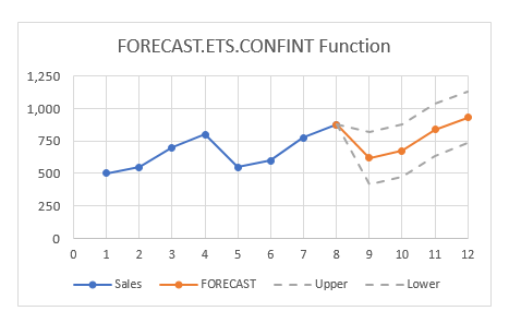
Note: Cells D12, F12, and G12 are set equal to C12 to connect the existing values to the forecast values in the chart.
Argument notes
The target_date argument represents the point on the timeline that a confidence interval prediction should be calculated.
The values argument contains the dependent array or range of data, also called y values. These are existing historical values from which a prediction will be calculated.
The timeline argument is the independent array or range of values, also called x values. The timeline, must consist of numeric values with a constant step interval. For example, the timeline could be yearly, quarterly, monthly, daily, etc. The timeline can also be a simple list of numeric periods, as in the example shown.
The seasonality argument is optional and represents the length of the seasonal pattern expressed in timeline units. For example, in the example shown, data is quarterly, so seasonality is given as 4, since there are 4 quarters in a year, and the seasonal pattern is 1 year. Allowed values are 0 (no seasonality, use linear algorithm), 1 (calculate seasonal pattern automatically), and n (manual season length, a number between 2 and 8784, inclusive). The number 8784 = 366 x 24, the number of hours in a leap year.
The data_completion argument is optional and specifies how FORECAST.ETS.CONFINT should handle missing data points. The options are 1 (default) and zero. By default, FORECAST.ETS.CONFINT will provide missing data points by averaging neighboring data points. If zero is provided, FORECAST.ETS.CONFINT will treat missing data points as zero.
The aggregation argument is optional, and controls what function is used to aggregate data points when the timeline contains duplicate values. The default is 1, which specifies AVERAGE. Other options are given in the table below.
Note: FORECAST.ETS.CONFINT results will be more accurate if aggregation is performed beforehand.
| Value | Behavior |
|---|---|
| 1 (or omitted) | AVERAGE |
| 2 | COUNT |
| 3 | COUNTA |
| 4 | MAX |
| 5 | MEDIAN |
| 6 | MIN |
| 7 | SUM |
Errors
The FORECAST.ETS.CONFINT function will return errors as shown below.
| Error | Cause |
|---|---|
| #VALUE! | target_date is not numeric seasonality is not numeric data_completion is not numeric aggregation is not numeric |
| #N/A | values and timeline are not the same size |
| #NUM | Consistent step cannot be determined in timeline All timeline values are the same The value for seasonality is not within 0-8784 The value for data_completion is not 0 or 1 The value for aggregation is not within 1-7 |
Purpose
Return value
Syntax
=FORECAST.ETS.SEASONALITY(values,timeline,[data_completion],[aggregation])
- values - Existing or historical values (y values).
- timeline - Numeric timeline values (x values).
- data_completion - [optional] Missing data treatment (0 = treat as zero, 1 = average). Default is 1.
- aggregation - [optional] Aggregation behavior. Default is 1 (AVERAGE). See other options below.
Using the FORECAST.ETS.SEASONALITY function
The FORECAST.ETS.SEASONALITY function returns the length in time of a seasonal pattern based on existing values and a timeline. FORECAST.ETS.SEASONALITY can be used to calculate the season length for numeric values like sales, inventory, expenses, etc. exhibit a seasonal pattern. If a pattern cannot be detected, FORECAST.ETS.SEASONALITY returns zero.
Example
In the example shown, the formula in cell H16 is:
=FORECAST.ETS.SEASONALITY(C5:C16,B5:B16)
where C5:C16 contains existing values, and B5:B16 contains a timeline. With these inputs, the FORECAST.ETS.SEASONALITY function returns 4. The result is 4 because the values in C5:C16 represent quarterly sales data, and the length of the season is 1 year, which is 4 quarters.
The chart to the right shows this data plotted in a scatter plot .
Argument notes
The values argument contains the dependent array or range of data, also called y values. These are existing historical values from which a season length will be calculated.
The timeline argument is the independent array or range of values, also called x values. The timeline must consist of numeric values with a constant step interval. For example, the timeline could be yearly, quarterly, monthly, daily, etc. The timeline can also be a simple list of numeric periods, as in the example shown.
The data_completion argument is optional and specifies how FORECAST.ETS.SEASONALITY should handle missing data points. The options are 1 (default) and zero. By default, FORECAST.ETS.SEASONALITY will provide missing data points by averaging neighboring data points. If zero is provided for data_completion, FORECAST.ETS.SEASONALITY will treat missing data points as zeros.
The aggregation argument is optional, and controls how the function should aggregate data points when the timeline contains duplicate timestamps. The default is 1, which specifies AVERAGE. Other options are given in the table below.
Note: It is better to perform aggregation before using FORECAST.ETS.SEASONALITY to make results as accurate as possible.
| Value | Behavior |
|---|---|
| 1 (or omitted) | AVERAGE |
| 2 | COUNT |
| 3 | COUNTA |
| 4 | MAX |
| 5 | MEDIAN |
| 6 | MIN |
| 7 | SUM |
Errors
The FORECAST.ETS.SEASONALITY function will return errors, as shown below.
| Error | Cause |
|---|---|
| #VALUE! | seasonality is not numeric data_completion is not numeric aggregation is not numeric |
| #N/A | values and timeline are not the same size |
| #NUM | Consistent step cannot be determined in timeline All timeline values are the same The value for data_completion is not 0 or 1 The value for aggregation is not within 1-7 |
