Details
The problem
There is one master test (Test A), and three variants (Test B, Test C, and Test D). All 4 tests have the same 19 questions, but arranged in a different order.
The first table in the screen below is a “question key” and shows how questions in Test A are ordered in the other 3 tests. The second table is an “answer key” that shows the correct answers for all 19 questions in all tests.

Above: Correct answers in I5:K23, formula obscured
For example, the answer to question #1 in Test A is C. This same question appears as question #4 in Test B, so the answer to question #4 in Test B is also C.
The first question in Test B is the same as question #13 in Test A, and the answer to both is E.
The challenge
What formula can be entered in I5 (that’s an i as in “igloo”) and copied across I5:K23 to find and display the correct answers for Tests B, C, and D?
You’ll find the Excel file below. Leave your answer as a comment below.
Hints
- This problem is challenging to set up. It’s very easy to get confused. Remember, the numbers in C5:E23 only tell you where you can find a given question. You still have to find the question after that :)
- This problem can be solved with INDEX and MATCH, which is explained in this article . Part of the solution involves carefully locking cell references. If you have trouble with these kind of references, practice building the multiplication table shown here . This problem requires carefully constructed cell references!
- You might find yourself thinking you could do this faster manually. Yes, for a small number of questions. However, with more questions (imagine 100, 500, 1000 questions) the manual approach gets much harder . A good formula will happily handle thousands of questions, and it won’t make mistakes :)
Details
The context
A couple weeks ago, I had an interesting question from a reader about tracking weight gain or loss in a simple table.
The idea is to enter a new weight each day, and calculate the difference from the previous day. When every day has an entry, the formula is straightforward:
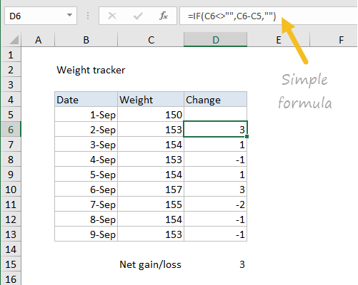
The difference is calculated with a formula like this, entered in D6, and copied down the table:
=IF(C6<>"",C6-C5,"")
However, when one or more days are missed, things go awry, and the calculated result doesn’t make sense:
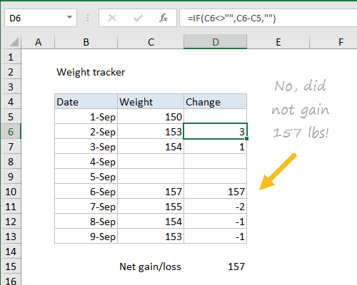
No, you did not gain 157 pounds in one day
The problem is the formula uses the blank cell in the calculation, which evaluates to zero. What we need is a way to locate and use the last weight recorded in column C.
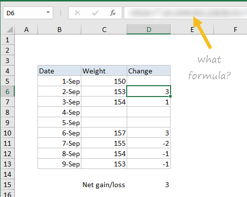
The challenge
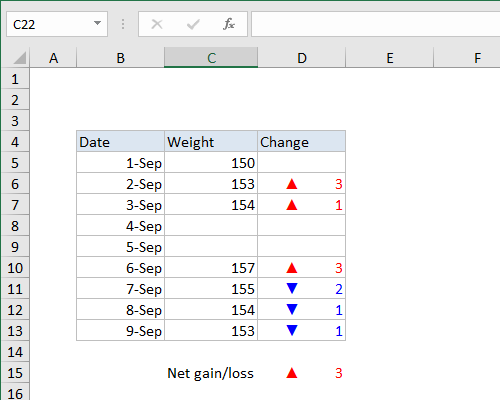
What formula will calculate a difference from the last entry, even when days have been skipped?
Desired result - difference using last previous entry
Assumptions
- A single formula is entered in D6 and copied down (i.e. same formula in all cells)
- The formula must handle one or many previous blank entries
- Removing blank entries (rows) is not allowed
- No helper columns allowed
Note: one obvious path is to use a Nested IF formula. I would discourage this, since it won’t scale well to handle an unknown number of consecutive blank entries.
I hacked together a formula myself, and I’ll share my solution after I give the smart readers of Exceljet some time to submit their own formulas.
Extra credit
Looking for more of a challenge? Here’s the same result, with a custom number format applied. What’s the number format? I swiped this from Mike Alexander on his now-defunct Bacon Bits blog.