In a world where everyday is Saturday or Sunday….
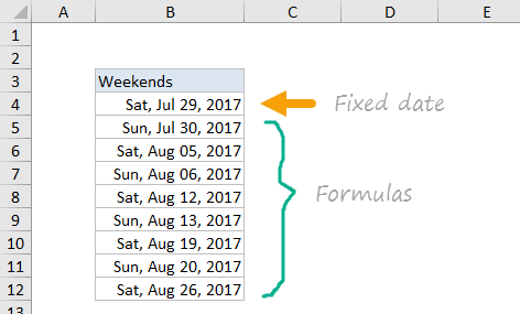
Here’s a little puzzle for you…how can you use Excel to generate a list of dates that are weekends only? For example, a list of Saturday Sunday pairs like this:
A couple years ago, I found and described a formula that will do it using the WEEKDAY function and some tricky date logic handled with IF:
=IF(WEEKDAY(A1)=7,A1+1,A1+(7-WEEKDAY(A1)))
With a date in A1, you can enter the formula in A2 and drag down to get your list of weekend dates.
This formula works fine, but it’s overly complicated. As a smart reader pointed out recently, you can do the same thing with the WORKDAY.INTL function and a much simpler formula:
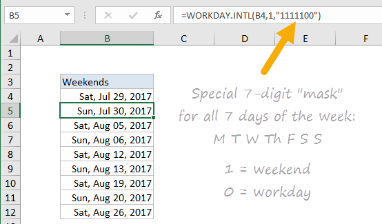
=WORKDAY.INTL(A1,1,"1111100")
This takes advantage of what I call the “mask” feature of WORKDAY.INTL, which allows you to designate any day of the week as a weekend. The logic may seem a little backwards, but basically 1 means “weekend” and 0 means “not weekend”. So, “1111100” effectively filters out all days except Saturday and Sunday by telling WORKDAY.INTL that Mon-Fri are weekends.
What I love about this example is how an initially complicated formula “collapses” into a simple solution.
Excel is full of hidden gems like this that can drastically simplify your work. The trick is of course is finding them :)
By the way, the NETWORKDAYS.INTL function also supports same 7-digit mask feature.
More formula info
- More about WORKDAY.INTL
- Calculate due dates with WORKDAY (video)
- More formula examples
- Excel formula training
One of the many cool things about Excel is that you can use formulas to display useful, dynamic messages directly on the worksheet. Dynamic messages give your spreadsheets a nice polish. Because they respond instantly to user input, the effect is friendly and professional:
A key tool in building friendly messages is concatenation . Concatenation sounds complicated, but it’s a really simple and useful formula technique you can learn in a few minutes. You’ll find many opportunities to use concatenation in your spreadsheets.
Caution: When people see messages like this in a worksheet you built, they’ll assume you’re some kind of Excel genius, so be warned :)
A basic example
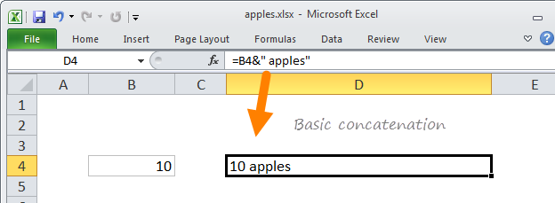
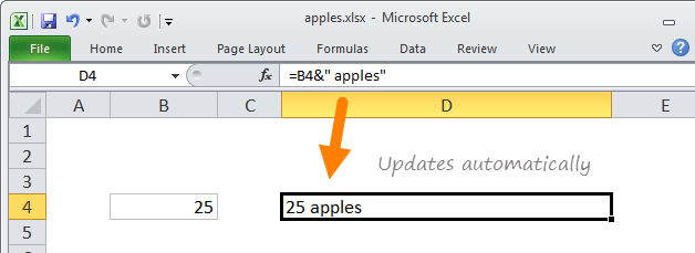
You can assemble messages with nothing more than a simple formula and a technique called “concatenation”. Don’t be alarmed by this fancy-sounding word. Concatenation simply means “join together”. In Excel, this generally means joining text with a value from a cell, or with the result of a function. For example, with the number 10 in cell B4, you can write a formula like this:
=B4&" apples"
Which displays this message: 10 apples
Note: text is fully enclosed in double quotes, and must include required spaces.
Here, the ampersand character (&) is used to join a text string with the value in cell A1. The ampersand is the “concatenation operator” in Excel, just like the asterisk (*) is the multiplication operator, the plus symbol (+) is the addition operator, and so on.
If a user updates cell B4 to contain 25, the message updates instantly:
Embedding a value in the middle
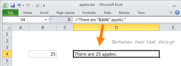
You don’t have to concatenate only at the beginning or end of a text string, you can use multiple ampersands to embed values anywhere you like in a string. Taking the example above another step, you can use two ampersands to create a full sentence with a value in the middle:
="There are "&B4&" apples."
Which returns: There are 25 apples.
Again note: all text must be enclosed in double quotes. If you forget to do this, Excel won’t let you enter the formula.
Concatenation with other functions
Once you get the basic idea of concatenation, you’ll quickly see how you can use the results of other formulas or functions in your messages. For example, perhaps you maintain data in a filtered table. You often use one or more filters to narrow down data in the table, and you’d like to know how many records you’re viewing at any given time, and how many records are in the table total.
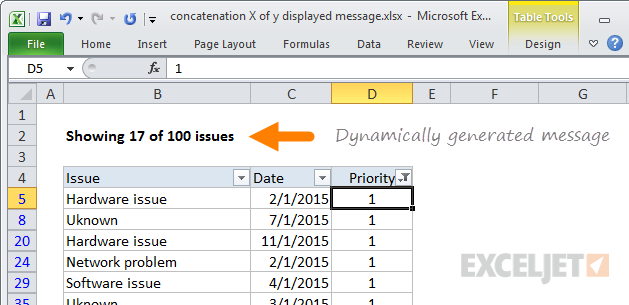
Building on the examples above, you can use concatenation, together with the row and subtotal functions to build a message like this: “Displaying x of y records”. Here, x represents the total record count, and y is the number of records currently visible, as seen below:
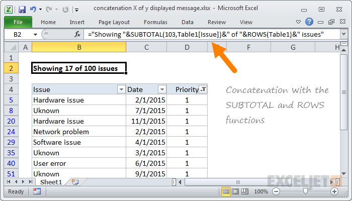
The formula used is:
="Showing "&SUBTOTAL(103,Table1[Issue])&" of "&ROWS(Table1)&" issues"
Video: How to count items in a filtered list
Concatenation with number formatting
Once you get comfortable with concatenation, you’ll start to notice many opportunities to concatenate values into more meaningful messages. Then, one of the first problems you’ll likely run into is losing the formatting of numeric values you include in a message.
For example, let’s say you have a due date in cell C4, and you want to display a message like “The project is due August 15, 2017”.
So, you start off with this formula:
="The project is due on "&C2
However, when you hit enter you see: The project is due on 42962
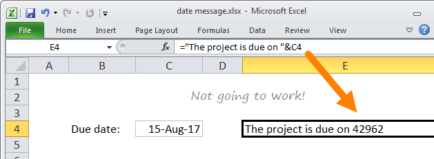
It’s kind of cool to see the underlying value, but most people don’t know that August 15, 2017 is the 42962-th day in Excel’s date numbering system, so not especially useful :)
To fix this problem, use the TEXT function to apply the formatting of your choice:
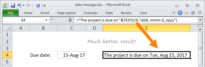
The improved version uses this formula:
="The project is due on "&TEXT(C2,"ddd, mmm d, yyyy")
The TEXT function is a handy function you can use whenever you want to apply formatting to a numeric value and up with text. You can use it for all number formatting, including percentage, currency, dates, times, and custom formats.
The video below shows how to use the TEXT function to increment a padded number (i.e. 0001, 00123, etc.)
Video: How to combine functions in a formula
Clarify assumptions with concatenation
Another cool use of concatenation is to make assumptions clear in a model that requires specific user inputs or variables.
This video below shows how concatenation can be used to “expose” several assumptions directly on the worksheet by concatenating variable inputs directly to calculation labels.
Video: How to clarify assumptions with concatenation
Excel concatenation functions
Excel contains three functions you can also use for concatenation: the CONCATENATE function , the CONCAT function , and the TEXTJOIN function . CONCAT and TEXTJOIN are new functions available in Office 365 and Excel 2019.
I’m not a fan of CONCATENATE, since it doesn’t do anything you can’t do with the regular old ampersand (&), which is much shorter, and more flexible to boot.
But CONCAT will let you join ranges, which is a new feature, and TEXTJOIN goes one step further and lets you join ranges with a delimiter of your choice. They are worth a look if you are using a newer version of Excel. This article discusses both functions in more detail: CONCAT and TEXTJOIN .
