Explanation
In this example, the goal is to create an “locked” reference that won’t change when columns or rows are added or deleted in a worksheet, or during a copy / paste / cut operation.
The INDIRECT function accepts text, and evaluates that text as a reference. As a result, the text is not susceptible to changes, like a normal cell reference. It will continue to evaluate to the same location regardless of changes to the worksheet. For example, this formula:
=INDIRECT("A1")
will continue to return a reference to cell A1 even if row 1, or column A, are deleted.
Examples
A reference created with INDIRECT can be used just like a regular cell reference in other formulas. In the worksheet shown above, the formulas in E5:E9 use INDIRECT to create a locked reference that won’t change:
=INDIRECT("B5")
=SUM(INDIRECT("B5:B16"))
=MIN(INDIRECT("B5:B16"))
=MAX(INDIRECT("B5:B16"))
=COUNT(INDIRECT("B5:B16"))
This approach can be useful when a worksheet is routinely edited in a way that would break traditional cell references.
Sheet names
Formulas with sheet names must follow standard rules. Sheets names without spaces or punctuation need no extra handling:
=INDIRECT("Sheet1!A1")
Sheet names with space or punctuation need to be enclosed in single quotes (’):
=INDIRECT("'Sheet 1'!A1") // note single quotes
Note: if you rename a sheet name used in INDIRECT, the reference will break. This happens because the reference is entered as text and therefore is not automatically updated like a normal reference.
Different from absolute and relative references
Using INDIRECT is different from standard absolute, relative, and mixed references . The $ syntax is designed to allow “intelligent” copying and pasting of formulas, so that references that need to change will change , while references that shouldn’t change, will not change . Using INDIRECT with text references stops all changes to the reference, even when columns/rows are inserted or deleted, or when a sheet is renamed.
Note: INDIRECT is a " volatile function " function, and can cause slow performance in large or complicated workbooks.
Explanation
Working from the inside out, the expression C5:G5<>"" returns an array of true and false values:
{FALSE,TRUE,FALSE,FALSE,FALSE}
The number 1 is divided by this array, which creates a new array composed of either 1’s or #DIV/0! errors:
{#DIV/0!,1,#DIV/0!,#DIV/0!,#DIV/0!}
This array is used as the lookup_vector.
The lookup_value is 2, but the largest value in the lookup_array is 1, so LOOKUP will match the last 1 in the array.
Finally, LOOKUP returns the corresponding value in result_vector, from the dates in the range C$4:G$4.
Note: the result in column H is a date from row 5, formatted with the custom format “mmm” to show an abbreviated month name only.
Zeros instead of blanks
You might have a table with zeros instead of blank cells:
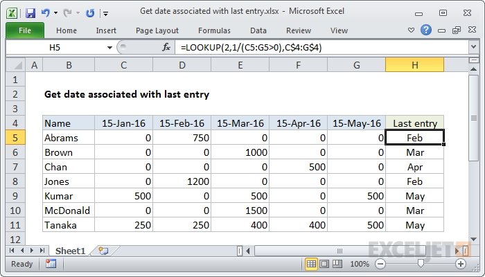
In that case, you can adjust the formula to match values greater than zero like so:
=LOOKUP(2,1/(C5:G5>0),C$4:G$4)
Multiple criteria
You can extend criteria by adding expressions to the denominator with boolean logic . For example, to match the last value greater than 400, you can use a formula like this:
=LOOKUP(2,1/((C5:G5<>"")*(C5:G5>400)),C$4:G$4)
