Explanation
Working from the inside out, the expression C5:G5<>"" returns an array of true and false values:
{FALSE,TRUE,FALSE,FALSE,FALSE}
The number 1 is divided by this array, which creates a new array composed of either 1’s or #DIV/0! errors:
{#DIV/0!,1,#DIV/0!,#DIV/0!,#DIV/0!}
This array is used as the lookup_vector.
The lookup_value is 2, but the largest value in the lookup_array is 1, so LOOKUP will match the last 1 in the array.
Finally, LOOKUP returns the corresponding value in result_vector, from the dates in the range C$4:G$4.
Note: the result in column H is a date from row 5, formatted with the custom format “mmm” to show an abbreviated month name only.
Zeros instead of blanks
You might have a table with zeros instead of blank cells:
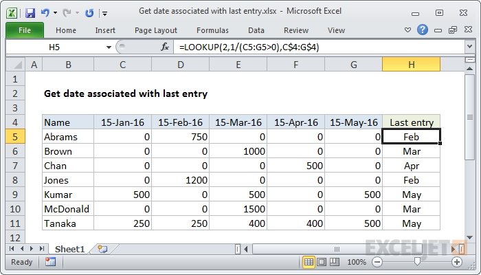
In that case, you can adjust the formula to match values greater than zero like so:
=LOOKUP(2,1/(C5:G5>0),C$4:G$4)
Multiple criteria
You can extend criteria by adding expressions to the denominator with boolean logic . For example, to match the last value greater than 400, you can use a formula like this:
=LOOKUP(2,1/((C5:G5<>"")*(C5:G5>400)),C$4:G$4)
Explanation
Note: the values in E5:E8 are actual dates, formatted with the custom number format “mmm”.
Working from the inside out, the expression:
MATCH(TRUE,TEXT(date,"mmyy")=TEXT(E5,"mmyy")
uses the TEXT function to generate an array of strings in the format “mmyy”:
{"0117";"0117";"0117";"0217";"0217";"0217";"0317";"0317";"0317"}
which are compared to a single string based on the value in E5, “0117”. The result is an array of TRUE / FALSE values:
{TRUE;TRUE;TRUE;FALSE;FALSE;FALSE;FALSE;FALSE;FALSE}
This array is fed into the MATCH function as the lookup_array , with a lookup_value of TRUE, and a match_type of zero for exact match. In exact match mode, the MATCH function returns the position of the first TRUE in the array, which is 1 in the formula in F5. This position goes into INDEX as the row number, with an array based on the named range “entry”:
=INDEX(entry,1)
Finally, INDEX returns the item inside entry as a final result.
Note: if an entry isn’t found for a given month and year, this formula will return #N/A.
Get the first entry based on today’s date
To get the first entry for a given month and year based on today’s date, you can adapt the formula to use the TODAY function instead of the value in E5:
{=INDEX(entry,MATCH(TRUE,TEXT(date,"mmyy")=TEXT(TODAY(),"mmyy"),0))}
