Explanation
The gist of this problem is that we want to get the first non-blank cell, but we don’t have a direct way to do that in Excel. The easiest way to solve this problem is with the XLOOKUP function.
XLOOKUP function
The XLOOKUP function is a modern upgrade to the VLOOKUP function. XLOOKUP is very flexible and can handle many different lookup scenarios. The generic syntax for required inputs looks like this:
=XLOOKUP(lookup_value,lookup_array,return_array)
The meaning of these arguments is as follows:
- lookup_value - the value to look for
- lookup_array - the range or array to search within
- return_array - the range or array to return values from
For more details, see How to use the XLOOKUP function .
The ISBLANK function
The ISBLANK function simply returns TRUE when a cell is empty, and FALSE if a cell is not empty. If A1 contains “apple” and B1 contains nothing, then ISBLANK returns the following:
=ISBLANK(A1) // returns FALSE
=ISBLANK(B1) // returns TRUE
For more details, see How to use the ISBLANK function .
NOT function
The NOT function simply returns the opposite of a given logical or Boolean value:
=NOT(FALSE) // returns TRUE
=NOT(TRUE) // returns FALSE
You can use the NOT function to “reverse” the output from other functions like ISBLANK, as seen below.
For more details, see How to use the NOT function .
XLOOKUP formula
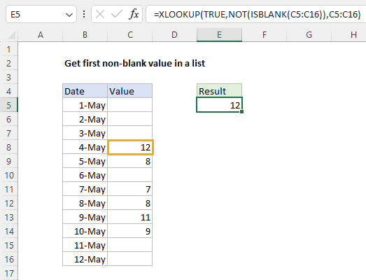
The formula in cell E5 combines the functions above like this:
=XLOOKUP(TRUE,NOT(ISBLANK(C5:C16)),C5:C16)
At a high level, XLOOKUP looks for TRUE and returns a corresponding value from C5:C16. It first uses ISBLANK to create an array with TRUE for blank cells and FALSE for non-blank cells. This array is then reversed using the NOT function, resulting in TRUE for non-blank cells and FALSE for blank cells. This final array serves as the lookup array for XLOOKUP. Working from the inside out, we start with the ISBLANK function is given the range C5:C16 like this:
ISBLANK(C5:C16)
Because C5:C16 contains 12 values, ISBLANK returns an array that contains 12 TRUE and FALSE results.
{TRUE;FALSE;TRUE;FALSE;FALSE;TRUE;FALSE;FALSE;FALSE;FALSE;TRUE;TRUE}
The TRUE values in the array indicate blank cells, and the FALSE values indicate non-blank cells. The array is returned directly to the NOT function in order to “reverse” the results. The output from NOT is a new array like this:
{FALSE;TRUE;FALSE;TRUE;TRUE;FALSE;TRUE;TRUE;TRUE;TRUE;FALSE;FALSE}
In this array, the TRUE values in the array indicate non-blank cells and the FALSE values indicate blank cells. This array is delivered directly to the XLOOKUP function as the lookup_array :
=XLOOKUP(TRUE,{FALSE;TRUE;FALSE;TRUE;TRUE;FALSE;TRUE;TRUE;TRUE;TRUE;FALSE;FALSE},C5:C16)
With a lookup value of TRUE, XLOOKUP matches the first TRUE in the lookup_array (the second value), and returns the corresponding value from the range C5:C16 (10) as a final result.
Testing the formula
To test the formula, we can delete the value in C6. The formula returns the value in cell C8 after the value in cell C6 is deleted:
More specific tests
You can easily adapt the XLOOKUP formula above to target certain types of content specifically. To find the first numeric value in a list, you can modify the XLOOKUP formula to use the ISNUMBER function :
=XLOOKUP(TRUE,ISNUMBER(range),range)
To find the first text value, use the ISTEXT function :
=XLOOKUP(TRUE,ISTEXT(range),range)
One quirk of ISBLANK is that it returns FALSE if a cell contains a formula that returns an empty string (""), even though an empty string is meant to look like a blank cell. If you need to detect cells that contain a formula returning an empty string (""), you can use the LEN function :
=XLOOKUP(TRUE,LEN(range)>0,range)
Technically, this formula is testing for cells that have more than zero characters.
INDEX and MATCH formula
In older versions of Excel that do not provide the XLOOKUP function, you can use an array formula based on INDEX and MATCH like this:
=INDEX(C5:C16,MATCH(TRUE,NOT(ISBLANK(C5:C16)),0))
Note: this is an array formula and must be entered with control + shift + enter in Excel 2019 and older.
This formula has basically the same logic as the XLOOKUP formula above. The MATCH function is used to find the position of the first non-blank cell in C5:C16. The NOT and ISBLANK functions create an array of TRUE (for non-blank cells) and FALSE (for blank cells) values that are used as a lookup array.
MATCH(TRUE,NOT(ISBLANK(C5:C16)),0)
After NOT and ISBLANK are evaluated, we have an array like this:
{FALSE;TRUE;FALSE;TRUE;TRUE;FALSE;TRUE;TRUE;TRUE;TRUE;FALSE;FALSE}
The array is returned to the MATCH function as the lookup_array . The lookup_value is provided as TRUE, and match_type is set to 0 to force an exact match:
MATCH(TRUE,{FALSE;TRUE;FALSE;TRUE;TRUE;FALSE;TRUE;TRUE;TRUE;TRUE;FALSE;FALSE},0)
MATCH then returns the location of the first TRUE in the array (2) as the row number to INDEX:
=INDEX(C5:C16,2) // returns 10
INDEX takes over and returns the value from the second cell in C5:C16 (10) as a final result.
As with XLOOKUP above, you can adapt the INDEX and MATCH formula to target specific content. For example, to get the first numeric value, use ISNUMBER:
=INDEX(range,MATCH(TRUE,ISNUMBER(range),0)) // first number
To get the first text value, use ISTEXT:
=INDEX(range,MATCH(TRUE,ISTEXT(range),0)) // first text
To get the value in the first cell with more than zero characters, use LEN:
=INDEX(range,MATCH(TRUE,LEN(range)>0,0))
These are all array formulas, which must be entered with control + shift + enter in Excel 2019 and older.
For more details, see How to use INDEX and MATCH .
Explanation
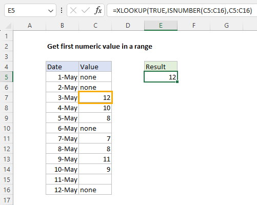
The general goal is to return the first numeric value in a row or column. More specifically, in the worksheet shown, we have dates in column B and a numeric value in the range C5:C16. Notice that all of the cells in this range have numeric values. Some are blank and some contain text values. We want the first number that appears in the range C5:C16. This problem can be solved using the XLOOKUP function or, in older versions of Excel, an INDEX and MATCH formula. Both methods are explained below.
XLOOKUP function
The XLOOKUP function is a modern upgrade to the VLOOKUP function. XLOOKUP is flexible and can handle many different lookup scenarios. The generic syntax for required inputs looks like this:
=XLOOKUP(lookup_value,lookup_array,return_array)
Where each argument has the following meaning:
- lookup_value - the value to look for
- lookup_array - the range or array to search within
- return_array - the range or array to return values from
For more details, see How to use the XLOOKUP function .
The ISNUMBER function
The ISNUMBER function returns TRUE when a cell contains a number, and FALSE if a cell is empty or contains a text value. If A1 contains “Age”, A2 contains 32, and cell A3 is empty, the ISNUMBER function returns the following:
=ISNUMBER(A1) // returns FALSE
=ISNUMBER(A2) // returns TRUE
=ISNUMBER(A3) // returns FALSE
For more details, see How to use the ISNUMBER function .
XLOOKUP formula
In the worksheet shown, the formula in cell E5 combined XLOOKUP and ISNUMBER like this:
=XLOOKUP(TRUE,ISNUMBER(C5:C16),C5:C16)
At a high level, the XLOOKUP function is configured with the lookup_value set to TRUE. The lookup_array is generated with the ISNUMBER function here:
ISNUMBER(C5:C16)
Because the range C5:C16 contains 12 cells, ISNUMBER returns an array that contains 12 TRUE and FALSE results like this:
{FALSE;FALSE;FALSE;TRUE;TRUE;FALSE;TRUE;TRUE;TRUE;TRUE;FALSE;FALSE}
The TRUE values in this array indicate cells that contain numbers. The FALSE values indicate cells that either contain text values or are empty, such as cell C16. This array is then returned directly to the XLOOKUP function as the lookup_array . At this point, we have the following:
=XLOOKUP(TRUE,{FALSE;FALSE;FALSE;TRUE;TRUE;FALSE;TRUE;TRUE;TRUE;TRUE;FALSE;FALSE},C5:C16)
With a lookup value of TRUE, XLOOKUP matches the first TRUE in the lookup_array (the fourth value), and returns the corresponding value from the range C5:C16 (10) as a final result.
Testing the formula
This formula is dynamic and will always return the first numeric value. To test the formula, we can add the number 12 to cell C7. Now the formula returns the 12, since 12 becomes the first numeric value in the range C5:C16.
INDEX and MATCH formula
In older versions of Excel that do not provide the XLOOKUP function, you can use an array formula based on INDEX and MATCH like this:
=INDEX(C5:C16,MATCH(TRUE,ISNUMBER(C5:C16),0))
Note: this is an array formula and must be entered with control + shift + enter in Excel 2019 and older.
This formula uses the same logic as the XLOOKUP formula above. The MATCH function is used to find the position of the first numeric value in C5:C16.
MATCH(TRUE,ISNUMBER(C5:C16),0)
The ISNUMBER function returns an array of TRUE (numeric) and FALSE (not numeric) values:
{FALSE;FALSE;FALSE;TRUE;TRUE;FALSE;TRUE;TRUE;TRUE;TRUE;FALSE;FALSE}
The array is returned to the MATCH function as the lookup_array . The lookup_value is given as TRUE and match_type is set to 0 to require an exact match:
MATCH(TRUE,{FALSE;FALSE;FALSE;TRUE;TRUE;FALSE;TRUE;TRUE;TRUE;TRUE;FALSE;FALSE},0)
MATCH then returns the location of the first TRUE in the array (4) as the row number to INDEX:
=INDEX(C5:C16,4) // returns 10
INDEX then returns the value from the fourth cell in C5:C16 (10) as a final result.
For more details, see How to use INDEX and MATCH .
