Explanation
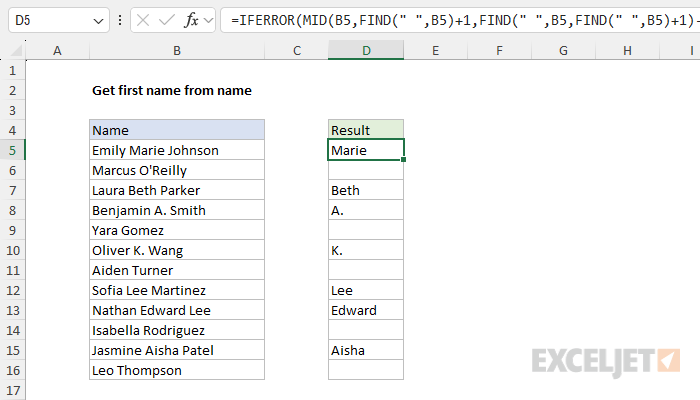
In this example, the goal is to return the middle name from a full name in “First Middle Last” format. In the current version of Excel this is a fairly simple problem using the TEXTAFTER and TEXTBEFORE functions. In older versions of Excel, a similar formula is significantly more complicated, based on the MID function and multiple FIND functions. Both approaches are explained below.
Modern solution
In the latest version of Excel you can solve this problem with the TEXTAFTER and TEXTBEFORE functions like this:
=TEXTAFTER(TEXTBEFORE(B5," ",-1)," ",,,,"")
As the formula is copied down, it returns the middle name when present, and an empty string ("") when there is no middle name. Working from the inside out, the TEXTBEFORE function is first used to extract all text that occurs after the last space in the name:
TEXTBEFORE(B5," ",-1) // returns "Emily Marie"
- text - the full name in cell B5
- delimiter - a single space (" “)
- instance_num - provided as -1 (first space from the end)
The trick here is using -1 for instance_num . A positive instance number tells TEXTBEFORE to count from the start of the text string. A negative instance number tells TEXTBEFORE to count from the end . The result is “Emily Marie” (the name without the last name) which is delivered to the TEXTAFTER function :
=TEXTAFTER("Emily Marie"," ",,,,"")
- text - result from TEXTBEFORE
- delimiter - a single space (” “)
- instance_num - omitted, defaults to 1
- match_mode - omitted
- match_end - omitted
- if_not_found - an empty string (”")
Essentially, we are asking TEXTAFTER for the text after the (first) space. Importantly, we also provide an empty string ("") for the if_not_found argument to gracefully handle cases where there is no middle name.
Legacy solution
In older versions of Excel that do not provide the TEXTAFTER or TEXTBEFORE functions, it is possible to use a more complex formula to extract the middle name:
=MID(B9,FIND(" ",B9)+1,FIND(" ",B9,FIND(" ",B9)+1)-FIND(" ",B9)-1)
This Excel formula is designed to extract the text between the first and second space characters in the cell B5. At a high level, we are using the MID function to extract a substring from the text in cell B5, where the start_num is the position to start the extraction, and num_chars is the number of characters to extract:
MID(B5,start_num,num_chars)
The challenge is in working out the correct values for start_num and num_chars . To calculate a start number, we use the FIND function like this:
FIND(" ",B5)+1 // start_num
This finds the position of the first space in B5 and adds 1. This calculation is used to set the start_num for the MID function, effectively starting the extraction from the character immediately after the first space. Next, we need to calculate the number of characters to extract. This is a more difficult problem. First, we find the position of the second space in B5 like this:
FIND(" ",B5,FIND(" ",B5)+1)
Here, we take advantage of the fact that the FIND function has as optional third argument called start_num , which controls where FIND begins its search. When no value is provided, start_num will default to 1 and FIND will begin searching from the beginning of the text string. To find the second space , we are asking FIND to begin searching one character after the first space :
FIND(" ",B5)+1 // one char after first space
Once we know the location of the second space, we need to subtract the location of the first space:
FIND(" ",B5,FIND(" ",B5)+ )-FIND(" ",B5)-1
This code calculates the number of characters between the first and second space by subtracting the position of the first space from the position of the second space and then subtracting 1. The result is delivered to the MID function as the num_chars argument, and MID then extracts all text between the two spaces.
=MID(B5,FIND(" ",B5)+1,FIND(" ",B5,FIND(" ",B5)+1)-FIND(" ",B5)-1)
=MID(B5,7,FIND(" ",B5,FIND(" ",B5)+1)-FIND(" ",B5)-1)
=MID(B5,7,FIND(" ",B5,FIND(" ",B5)+1)-FIND(" ",B5)-1)
=MID(B5,7,FIND(" ",B5,6+1)-6-1)
=MID(B5,7,FIND(" ",B5,7)-6-1)
=MID(B5,7,12-6-1)
=MID(B5,7,5)
="Marie"
The formula above will work correctly when there are two spaces in the name. However, when a second space is not found (i.e. there is no middle name, FIND will return a #VALUE! error. An easy way to manage this error is to embed the original formula into the IFERROR function:
=IFERROR(MID(B5,FIND(" ",B5)+1,FIND(" ",B5,FIND(" ",B5)+1)-FIND(" ",B5)-1),"")
Now when a second space is not found, FIND will return a #VALUE! error, and IFERROR will catch that error and return an empty string (""), which looks like a blank cell in Excel.
Explanation
In this example, the goal is to join different parts of a name (first, middle, last) into a full name. This is an example of concatenation . To concatenate means to join one text value to another with a formula, or in a more general programming language. In a current version of Excel, the simplest approach is to use the TEXTJOIN function, which is a flexible function for concatenating values in Excel. In an older version of Excel, you can use manual concatenation with the ampersand (&) operator, or you can use the older CONCATENATE function. The article below discusses all three approaches.
Note: Formulas that use concatenation in Excel are quite common, so it is a skill worth knowing. For a more detailed explanation of concatenation see How to concatenate in Excel .
TEXTJOIN solution
In the current version of Excel, the easiest way to join different parts of a name together is to use the TEXTJOIN function . To join the First name in column B to the Last name in column D together with TEXTJOIN the formula in cell F5 looks like this:
=TEXTJOIN(" ",1,B5,D5)
The inputs to TEXTJOIN are as follows:
- delimiter - a single space (" “)
- ignore_empty - 1, equivalent to TRUE
- text1 - B5, the first name
- text2 - D5, the last name
With this configuration, TEXTJOIN joins the first name in cell B5 to the last name in cell D5 together with a single space (” “) between them. If either value is empty, the ignore_empty argument set to 1 will cause TEXTJOIN to ignore the empty value and return the other value without a space.
You can easily adapt this formula to join all three names (first, middle, and last) together with TEXTJOIN. The formula used to perform this task in H5 looks like this:
=TEXTJOIN(" ",1,B5:D5)
- delimiter - a single space (” “)
- ignore_empty - 1, equivalent to TRUE
- text1 - the range B5:D5
Note that in this case, we give TEXTJOIN the range B5:D5 as text1 . TEXTJOIN will join all three values together separated by a single space (” “). Because ignore_empty is set to 1 (equivalent to TRUE in Excel), when a middle name is not present, TEXTJOIN will ignore that value and not add an extra space between the first and last names.
Note: newer versions of Excel also offer the CONCAT function (which replaces the CONCATENATE function in functionality). However, in this case, the TEXTJOIN function is a better option because it can automatically ignore empty values.
Manual concatenation solution
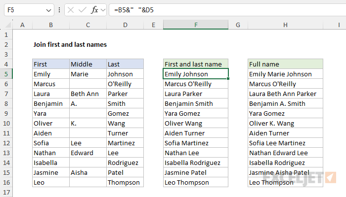
In an older version of Excel that does not offer the TEXTJOIN function, you can use manual concatenation with the ampersand (&) operator . This is often the technique used by more advanced users because it is simple and flexible. To join the first name in column B to the last name in column D together, you can use a formula like this:
=B5&" "&D5
The result is the first name in cell B5 joined to the last name in cell D5 separated by a space (” “). To use the manual concatenation to join the first, middle, and last names together, the formula in H5 is a bit more complex:
=B5&" "&IF(C5<>"",C5&" ","")&D5
At the core, this formula is similar to the first formula above. We begin with the first name in B5 and end with the last name in cell D5. However, to avoid adding an extra space when the middle name is blank we use the IF function to apply some conditional logic like this:
IF(C5<>"",C5&" ","")
The translation for this formula is: If cell C5 is not empty, return the value in C5 joined to a single space. If C5 is empty, return an empty string (”"). In other words, if there is a middle name, add it with a space, otherwise, add nothing.
Note: When you use concatenation in a formula, be sure to enclose any literal text in double quotes (""). However, do not enclose the ampersand (&) or cell references in quotes .
CONCATENATE solution
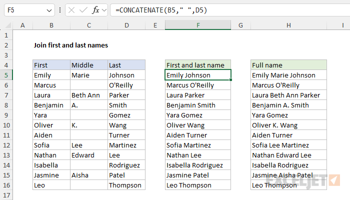
Another way to solve this problem is with the older CONCATENATE function . In the worksheet below the formula in cell F5 is:
=CONCATENATE(B5," ",D5)
And the formula in H5 looks like this:
=CONCATENATE(B5," ",IF(C5<>"",C5&" ",""),D5)
In the formula above, we aren’t able to avoid using the ampersand (&) entirely, because we still need the conditional logic created by the IF function to avoid adding extra space when the middle name is not present. This is something that TEXTJOIN handles automatically, which makes it a better option in more current versions of Excel.
