Explanation
In this example, the goal is to calculate the number of months between two valid Excel dates . This is a curiously tricky problem in Excel because the number of days in a month varies, and the rules about how a whole month might be calculated are not obvious. In addition, there is not a modern Excel function dedicated to the task of calculating months between dates. I have no idea why. The best tool for the job is the mysterious DATEDIF function, which is kind of a black sheep in the Excel family.
The DATEDIF function
The solutions described below are based primarily on the DATEDIF function. DATEDIF (date + dif) is designed to calculate the difference between a start date and an end date in years, months, or days. DATEDIF takes 3 arguments: start_date , end_date , and unit and the generic syntax looks like this:
=DATEDIF(start_date,end_date,unit)
For this problem, the start dates come from column B and the end dates come from column C. For unit, we need to supply “m”, because we want to calculate months between dates. See this page on the DATEDIF function for more information about the options available.
DATEDIF is a “compatibility” function that comes originally from Lotus 1-2-3. You can use DATEDIF in all current Excel versions, but you must enter the function manually — unlike other functions, DATEDIF will not appear as a suggested function in the formula bar and Excel will not help you with function arguments.
Calculate complete whole months
In the worksheet shown below, we are using the DATEDIF function to calculate complete whole months between a start date and an end date. The start dates come from column B and the end dates come from column C. The formula in D5, copied down, is:
=DATEDIF(B5,C5,"m")
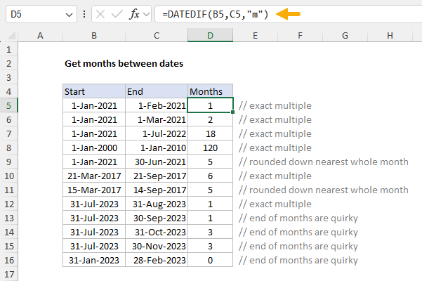
As the formula is copied down, DATEDIF returns whole months between the start date in column B and the end date in column C. Notice that the first four results in D5:D8 are exact multiples of months, but the result in D9 has been rounded down to 5 because we are 1 day short of 6 months. Also notice that results in D13:D16 are a bit quirky, due to how DATEDIF handles end-of-month dates. For example, when the days match, the result is an exact multiple of months, as expected. However, when the days don’t match, the results can be unexpected. For example, with a start date of July 31 and an end date of September 30, the result is 1, though most people would count this as 2 months. One workaround to this problem is described below.
Calculate nearest whole months
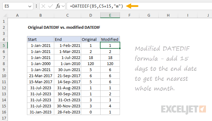
When calculating months between two dates, DATEDIF always rounds months down to the last complete number of months. This means DATEDIF rounds a result down even when it is very close to the next whole month. To calculate months to the nearest whole month, you can adjust the formula as shown below:
=DATEDIF(start_date,end_date+15,"m")
In this version of the formula, we add 15 days to the end date. This ensures that end dates in the second half of the month are treated like dates in the following month, effectively rounding up the final result to the next even multiple. End dates that occur in the first half of the month also increase by 15 days, but not enough to affect the normal result from DATEDIF. The screen below shows how the original DATEDIF formula compares to the modified version:
Calculate decimal months
As shown above, DATEDIF only calculates whole months. To calculate a decimal number that represents the number of months between two dates, you can use the YEARFRAC function like this:
=YEARFRAC(start,end)*12
YEARFRAC returns fractional years between two dates, so the result is an approximate number of months between two dates, including fractional months returned as a decimal value. The screen below shows how the original DATEDIF formula compares to the YEARFRAC version:

Keep in mind that the behavior of this formula depends on how YEARFRAC works. See this page for more information.
Alternative formula to calculate months touched by dates
In some cases, you may want to count how many months are “touched” by a given date range. The generic formula for this calculation looks like this:
=(YEAR(C5)-YEAR(B5))*12+MONTH(C5)-MONTH(B5)+1
This formula uses the YEAR function and the MONTH function to work out a count in two parts. First, the months associated with a year change are calculated:
(YEAR(end)-YEAR(start))*12 // months due to year change
This code only affects the count if the start year and end year are different. If the start year and end year are the same, the result is zero. Next, the formula subtracts the start month from the end month and adds 1 to calculate the remaining months:
MONTH(end)-MONTH(start)+1 // remaining months
Notice this calculation means that any month difference will result in a positive number because the day of the month is completely ignored. Finally, the two parts of the formula are added together to get a total month count. The screen below shows the formula in action, compared to the original DATEDIF formula above:
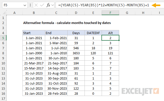
As you would expect, this formula tends to increase the month count for a date range, since even a small portion of a month will be included in the result. You can see this effect if you compare results from the original DATEDIF formula in column E to results from the alternative formula in column F.
Explanation
In this example, the goal is to create a formula that will return the most recent day of the week, given a date and a target day of the week, abbreviated as “dow” in the generic formula. Excel tracks the day of the week internally as a specific number for each of the seven days. By default, Excel assigns 1 to Sunday and 7 to Saturday as seen below:
| Day of week | Number |
|---|---|
| Sunday | 1 |
| Monday | 2 |
| Tuesday | 3 |
| Wednesday | 4 |
| Thursday | 5 |
| Friday | 6 |
| Saturday | 7 |
The formula solution
The generic version of the formula looks like this:
=date-MOD(date-dow,7)
In the example shown, cell B5 contains the date 1/16/2015, and the formula in D5 is:
=B5-MOD(B5-7,7)
The number 7 is the target dow (day of week). Excel first subtracts the dow (7 in this case) from the date, then feeds the result into the MOD function as the number with 7 as the divisor. MOD returns the remainder after division, which is subtracted from the start date. At a high level, the formula works like this:
- date - dow - Shifts the original date back by dow days to create a reference point in the past.
- MOD(date - dow, 7) - Normalizes the shift to a value within the current week (0-6 days). This value represents how many days back we are from a complete week cycle.
- B5-MOD(B5-7,7) - Subtracting the normalized value from the original date gives the most recent target day of the week.
The code below shows how Excel evaluates the formula step-by-step:
=B5-MOD(B5-7,7)
=B5-MOD(42020-7,7)
=B5-MOD(42013,7)
=B5-6
=42014 // 10-Jan-2015, a Saturday
The result is 42014, which is January 10, 2015, (a Saturday) in Excel’s date system.
Most recent day of the week today
If you want to get the most recent day of the week from the current date, you can use the TODAY function like this:
=TODAY()-MOD(TODAY()-dow,7)
Note: If the date is already the target day of the week, the date will be returned unchanged.
