Explanation
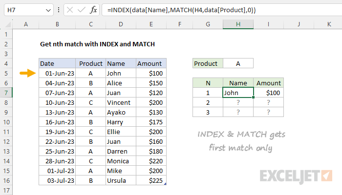
The goal is to retrieve the nth matching record in a table when targeting a specific product. For example, if the value in cell H4 is “A”, the formula in H7 should return the name “John”, since this is the first name in the table associated with product “A”. In the same way, the formula in H8 should return ‘Juan’, since this is the second name associated with product “A”. The product in H4 is an input that can be changed at any time. All data exists in an Excel Table named data .
Basic INDEX and MATCH
Before we look at the formula used in the worksheet, we should review why we can’t use a “normal” INDEX and MATCH formula to solve this problem. Normally, the INDEX and MATCH functions are used to find the position of a value in a table and return a corresponding value in the same position from a different column. However, this method only works for the first match. For example, in the screen below, these the INDEX and MATCH formulas in H7 and I7 are as follows:
=INDEX(data[Name],MATCH(H4,data[Product],0)) // returns "John"
=INDEX(data[Amount],MATCH(H4,data[Product],0)) // returns 100
In these formulas, the MATCH function is configured to match the value in H4 (“A”), in the Product column. In both formulas, MATCH returns 1 because the product is “A”. These formulas work perfectly, but the problem is that we have no way to ask MATCH to find the 2nd match, the 3rd match, etc.
As mentioned, this is a standard application of INDEX and MATCH. For a complete overview, see: How to use INDEX and MATCH .
INDEX and SMALL + IF
One workaround to the INDEX and MATCH limitation explained above is to use INDEX with the SMALL and IF instead of MATCH. At the core, this approach uses INDEX to get the name at a specific row number like this:
=INDEX(data[Name],row_num)
The challenge is how to calculate the row number for each nth match since MATCH will only find the first match. One workaround is to generate a set of row numbers for the entire table, then use the IF function to “filter” the row numbers based on the product specified in cell H4. Then we can give this filtered list to the SMALL function, which is designed to get the “nth smallest” value. That is the approach seen in the worksheet as shown, where the formula in H7 is as follows:
=INDEX(data[Name],SMALL(IF(data[Product]=$H$4,ROW(data)-MIN(ROW(data))+1),G7))
Note this is an array formula that must be entered with control + shift + enter in Excel 2019 and earlier.
All of the hard work in this formula is in determining a row number for INDEX, which is done here:
SMALL(IF(data[Product]=$H$4,ROW(data)-MIN(ROW(data))+1),G7)
This may look complicated, but the approach is pretty straightforward. We create row numbers for the data, filter the numbers with an appropriate logical test, then retrieve the nth matching row number. Working from the inside out, the code below generates a set of relative row numbers for the entire table:
ROW(data)-MIN(ROW(data))+1
Since there are 12 rows in the table, the result is an array like this:
{1;2;3;4;5;6;7;8;9;10;11;12}
For more details on how this works, see this page . Simplifying the formula, we now have:
SMALL(IF(data[Product]=$H$4,{1;2;3;4;5;6;7;8;9;10;11;12}),G7)
Next, the IF function applies a logical test to filter on numbers where the product is “A” in H4:
IF(data[Product]=$H$4,{1;2;3;4;5;6;7;8;9;10;11;12})
Because there are 12 rows in the table, the result is an array like this:
{1;FALSE;3;FALSE;5;FALSE;FALSE;FALSE;9;FALSE;11;FALSE}
Notice the only numbers to survive the filtering are the rows associated with product “A”. The other row numbers have been replaced by FALSE. Next, the SMALL function is used to return the nth smallest value:
SMALL({1;FALSE;3;FALSE;5;FALSE;FALSE;FALSE;9;FALSE;11;FALSE},G7)
SMALL automatically ignores the FALSE values. With 1 in cell G7, SMALL returns the smallest value, which is 1. This is returned directly to the INDEX function as row_num . Back in the original formula, we now have:
=INDEX(data[Name],1) // returns "John"
The INDEX function then returns “John” in cell H7. In cell H8, the value in G8 is 2, and SMALL returns the second smallest row number, which is 3:
=INDEX(data[Name],3) // returns "Juan"
As the formula is copied down, the value for n increases in column G causing the SMALL function to retrieve the next matching row number. At each new row, the formula returns the next nth match.
Retrieving Amount
The formula to retrieve the associated Amount is almost exactly the same as the formula above:
=INDEX(data[Amount],SMALL(IF(data[Product]=$H$4,ROW(data)-MIN(ROW(data))+1),G7))
The only difference is the value for the array provided to INDEX, which is data[Amount] instead of data[Name] .
Handling errors
Once there are no more matches for a given value of n, the SMALL function will return a #NUM error. You can handle this error with the IFERROR function , or by adding logic to count matches and abort processing once the number in column H is greater than the match count. The example here shows one approach.
Multiple criteria
To add multiple criteria, you use boolean logic , as explained in this example .
Explanation
The table contains basic order information, with columns for Date, Product, Name, and Amount. The Helper column is used to create a special lookup value, as explained below. The goal is to retrieve the nth matching record in a table for a specific product, which is entered in cell I4. For example, if the value in cell H4 is “A”, the formula in I7 should return the name “John”, since this is the first name in the table associated with product “A”. In the same way, the formula in I8 should return ‘Juan’, since this is the second name associated with product “A”. If the product in H4 is changed, the formula should calculate a new result. All data exists in an Excel Table named data .
Helper column
This formula depends on a helper column , which is added as the first column to the source data table. The helper column uses a formula to create a unique ID to use as a lookup value using the product in column D and a counter created with the COUNTIF function . The lookup value is created by concatenating the product in I4 to a running count of the product. The formula in B5 is:
=D5&"-"&COUNTIF($D$5:D5,D5)
This formula picks up the value in D5 and uses the ampersand (&) to concatenate the product to a hyphen (-), and the result from COUNTIF. The COUNTIF function uses an expanding range ($D$5:D5) to generate a running count of the product in the table. The values in column B show the results of this formula.
VLOOKUP function
VLOOKUP is an Excel function to get data from a table organized vertically , with lookup values in the first column . The data to retrieve is specified by column number, and the generic syntax for VLOOKUP looks like this:
=VLOOKUP(lookup_value,table_array,column_index_num,range_lookup)
In this example, we use the formulas below to look up the name and amount for each match in the table:
=VLOOKUP($I$4&"-"&$H7,data,4,0) // name
=VLOOKUP($I$4&"-"&$H7,data,5,0) // amount
The lookup_value is the value to search for, and this is the tr icky part of this approach. To match the lookup values in column B, we need to create a lookup value in the same format as the IDs we created in the Helper column: a product code joined to a count, separated by a hyphen (i.e., “A-1”, “A-2”, etc.). To do this, we use the snippet below:
$I$4&"-"&$H7
Notice the reference to $I$4 is absolute so that it will not change when the formula is copied, while the reference to $H7 is mixed so that the column is locked but the row can change. As the formula is copied down, the lookup_value increments at each row using the numbers in column H. This is how the formula can return the first match, the second match, and so on.
The table_array is the Excel Table named data. Next, we have the column number, which is a number that indicates the column from which we want to retrieve data, where the first column is column 1 and contains lookup values. To get the Name, we use 4 for column_index_num, and to get the Amount, we use 5. Finally, we have the last argument, range_lookup, for which we provide zero (0). Using zero (0) tells VLOOKUP to find an exact match for the ID. If the exact ID isn’t found, VLOOKUP will return the #N/A error.
As the VLOOKUP formulas are copied down, they return the first five matches for Product A as shown in the worksheet. In cells I7 and J7, the lookup values and results look like this:
=VLOOKUP("A-1",data,4,0) // returns "John"
=VLOOKUP("A-1",data,5,0) // returns 100
In cells I8 and J8, we have:
=VLOOKUP("A-2",data,4,0) // returns "Juan"
=VLOOKUP("A-2",data,5,0) // returns 120
And so on, as the formula is copied down.
For more information about VLOOKUP, see: How to use the VLOOKUP function .
