Purpose
Return value
Syntax
=GETPIVOTDATA(data_field,pivot_table,[field1, item1],...)
- data_field - The name of the value field to query.
- pivot_table - A reference to any cell in the pivot table to query.
- field1, item1 - [optional] A field/item pair.
Using the GETPIVOTDATA function
Use the GETPIVOTDATA function to query an existing Pivot Table and retrieve specific data based on the pivot table structure. The advantage of GETPIVOTDATA over a simple cell reference is that it collects data based on structure , not cell location. GETPIVOTDATA will continue to work correctly even when a pivot table changes, as long as the field(s) being referenced is still present.
The first argument, data_field , names a value field to query. The second argument, pivot_t a ble, is a reference to any cell in an existing pivot table. Additional arguments are supplied in field/item pairs that act like filters to limit the data retrieved based on the structure of the pivot table. For example, you might supply the field “Region” with the item “East” to limit sales data to Sales in the East Region.
The GETPIVOTDATA function is generated automatically when you reference a value cell in a pivot table by pointing and clicking. To avoid this, you can simply type the address of the cell you want (instead of clicking). If you want to disable this feature entirely, disable “Generate GETPIVOTDATA” in the menu at Pivot TableTools > Options > Options (far left, below the pivot table name).
Examples
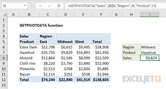
The examples below are based on the following pivot table:
The first argument in the GETPIVOTDATA function names the field from which to retrieve data. The second argument is a reference to a cell that is part of the pivot table. To get total Sales from the pivot table shown:
=GETPIVOTDATA("Sales",$B$4) // returns 138602
Fields and item pairs are supplied in pairs entered as text values . To get total sales for the Product Hazelnut:
=GETPIVOTDATA("Sales",$B$4,"Product","Hazelnut") // returns 62456
To get total Sales for the West region:
=GETPIVOTDATA("Sales",$B$4,"Region","West") // returns 41518
To get total sales for Almond in the East region, you can use either of the formulas below:
=GETPIVOTDATA("Sales",$B$4,"Region","East","Product","Almond")
=GETPIVOTDATA("Sales",$B$4,"Product","Almond","Region","East")
You can also use cell references to provide field and item names. In the example shown above, the formula in I8 is:
=GETPIVOTDATA("Sales",$B$4,"Region",I6,"Product",I7)
The values for Region and Product come from cells I5 and I6. The data is collected based on the region “Midwest” in cell I6 for the product “Hazelnut” in cell I7.
Dates and times
When using GETPIVOTDATA to fetch information from a pivot table based on a date or time date or time, use Excel’s native format , or a function like the DATE function . For example, to get total Sales on April 1, 2021 when individual dates are displayed:
=GETPIVOTDATA("Sales",A1,"Date",DATE(2021,4,1))
When dates are grouped , refer to the group names as text. For example, if the Date field is grouped by year:
=GETPIVOTDATA("Sales",A1,"Year","2021")
Notes
- The name of the data_field, and field/item values must be enclosed in double quotes (")
- GETPIVOTDATA will return a #REF error if any fields are spelled incorrectly.
- GETPIVOTDATA will return a #REF error if the reference to pivot_table is not valid.
Purpose
Return value
Syntax
=HLOOKUP(lookup_value,table_array,row_index,[range_lookup])
- lookup_value - The value to look up.
- table_array - The table from which to retrieve data.
- row_index - The row number from which to retrieve data.
- range_lookup - [optional] A Boolean to indicate exact match or approximate match. Default = TRUE = approximate match.
Using the HLOOKUP function
The HLOOKUP function can locate and retrieve a value from data in a horizontal table . Like the “V” in VLOOKUP which stands for “vertical”, the “H” in HLOOKUP stands for “horizontal”. The lookup values must appear in the first row of the table, moving horizontally to the right. HLOOKUP supports approximate and exact matching, and wildcards (* ?) for finding partial matches.
HLOOKUP searches for a value in the first row of a table. When it finds a match, it retrieves a value at that column from the row given. Use HLOOKUP when lookup values are located in the first row of a table. Use VLOOKUP when lookup values are located in the first column of a table.
HLOOKUP takes four arguments . The first argument, called lookup_value , is the value to look up. The second argument, table_array , is a range that contains the lookup table. The third argument, row_index_num is the row number in the table from which to retrieve a value. In the example shown, HLOOKUP is used to look up values from row 2 (Level) and row 3 (Bonus) in the table. The fourth and final argument, range_lookup , controls matching. Use TRUE or 1 for an approximate match and FALSE or 0 for an exact match.
Example #1 - approximate match
In the example shown, the goal is to look up the correct Level and Bonus for the sales amounts in C5:C13. The lookup table is in H4:J6, which is the named range “table”. Note this is an approximate match scenario. For each amount in C5:C13, the goal is to find the best match, not an exact match. To lookup Level, the formula in cell D5, copied down, is:
=HLOOKUP(C5,table,2,1) // get level
To get Bonus, the formula in E5, copied down, is:
=HLOOKUP(C5,table,3,1) // get bonus
Notice the only difference between the two formulas is the row index number: Level comes from row 2 in the lookup table, while Bonus comes from row 3. The match mode has been set explicitly to approximate match by providing the last argument, range_lookup , as 1.
Example #2 - exact match
In the screen below, the goal is to look up the correct level for a numeric rating 1-4. In cell D5, the HLOOKUP formula, copied down, is:
=HLOOKUP(C5,table,2,FALSE) // exact match

where table is the named range G4:J5. Notice the last argument, range_lookup is set to FALSE to require an exact match.
Notes
- Range_lookup controls whether the lookup value needs to match exactly or not. The default is TRUE = allow non-exact match.
- Set range_lookup to FALSE to require an exact match.
- If range_lookup is omitted or TRUE, and no exact match is found, HLOOKUP will match the nearest value in the table that is still less than the lookup value . However, HLOOKUP will still match an exact value if one exists.
- If range_lookup is TRUE , lookup values in the first row of the table must be sorted in ascending order. Otherwise, HLOOKUP may return an incorrect or unexpected value.
- If range_lookup is FALSE (exact match), values in the first row of the lookup table do not need to be sorted.
