Groupby With Monthly Totals

Explanation

In this example, the goal is to generate monthly totals using the GROUPBY function. This is a tricky problem in Excel because typically, source data contains a regular date field and not a separate field with month names. In addition, the GROUPBY function will, by default, sort everything in alphabetical order. This means when we add month names, they will sort A-Z and end up in the wrong order. Part of the challenge is figuring out the best way to sort the month names as part of the GROUPBY formula. To explain how this all works, let’s build the solution step by step.

Excel data for source data
The core GROUPBY formula
GROUPBY sort options
Adding the month numbers to sort by
Sorting the table by month number
Removing the month numbers
Summary of steps
Alternative formula #1
Alternative formula #2
Formula for older versions of Excel
Final thoughts

Excel data for source data

The source data is in an Excel Table named data in the range B4:E179, which contains daily sales data for the first 6 months of 2025. It’s not necessary to use an Excel table to solve this problem, but it makes the formula a bit easier to read and understand. Plus, it means that the solution is dynamic - if the source data is added or removed, the monthly subtotals will recalculate as needed.

Note: The source data contains only the first 6 months of 2025. This is to keep the example simple. The solution will work with any number of months.

The core GROUPBY formula

The GROUPBY function excels at grouping data. In this example, we’re going to use GROUPBY to group the data by month. The main challenge initially is that we don’t have month names in the data. We only have the raw dates. This means we need to create our own month names in the formula. An easy way to do that is to use the TEXT function, which allows us to generate month names any way we like using Excel’s custom number format codes. In this case, we will abbreviate the month names using the format code “mmm”. For example, with a date like 12-Jan-2025 in cell A1, TEXT would return “Jan”:

=TEXT("12-Jan-2025","mmm") // returns "Jan"

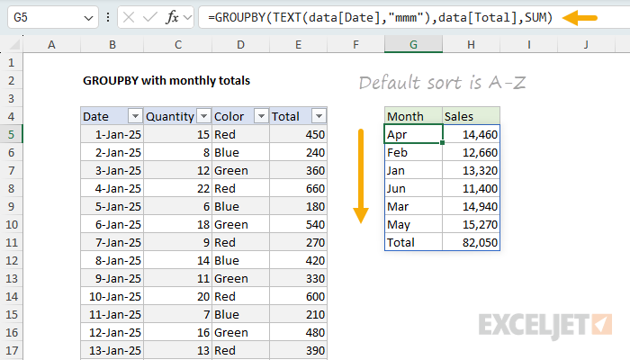
The complete formula in cell G5 below looks like this:

=GROUPBY(TEXT(data[Date],"mmm"),data[Total],SUM)

Excel worksheet showing GROUPBY results with monthly totals, but months are sorted alphabetically (Apr, Feb, Jan, Mar, May, Jun) instead of chronologically - 2

The first argument to GROUPBY is the data to group. Here we use the TEXT function to create the month names as shown above, with the code =TEXT(data[Date],“mmm”) . The result is a new column of month names derived directly from the dates. This column doesn’t actually exist in the source data, but we can use it as a row field in the GROUPBY function.
The second argument to GROUPBY is the data to aggregate. In this case, we want to aggregate the sales numbers in the Total column, so we use data[Total].
The third argument to GROUPBY is the function to use to aggregate the data. Because we want total sales per month, we want to use the SUM function.

This formula works nicely. You can see that we get a clean breakdown by month for the first six months of 2025. However, there is a problem. Notice that the month names do not appear in chronological order. Instead, they are sorted alphabetically. This is because the GROUPBY function sorts grouped values in alphabetical order by default.

GROUPBY sort options

By default, the GROUPBY function will sort values in standard ascending (A-Z) order, beginning with the leftmost row field. The result is that the month names are sorted alphabetically, starting with “Apr”. To override the default sort order, we can provide a value for the sort_order argument , which is given as an index number that can be positive (A-Z) or negative (Z-A). The number itself corresponds to the columns in the table, starting with 1 for the first column. For example, to sort the table by month name in descending (Z-A) order, we can provide -1 for sort_order in the GROUPBY function, like this:

=GROUPBY(TEXT(data[Date],"mmm"),data[Total],SUM,,,-1)

However, as you can see, that doesn’t help. The month names are still sorted alphabetically, but in reverse order, so now the first month name is “May” instead of “Apr”:

We’ll need to use a different approach.

Adding the month numbers to sort by

To sort the month names in chronological order, we need a different approach. The core problem is that we only have the month names as text, but what we need to sort in chronological order are month numbers . To get the month numbers, we can use the MONTH function, which returns the month number for a given date. For example, with a date like 12-Mar-2025, MONTH would return 3:

=MONTH("12-Mar-2025") // returns 3

We can get month numbers for all dates in the source data like this:

=MONTH(data[Date]) // returns 1-12 for all dates

Because there are 175 dates in the source data, this MONTH returns an array of 175 month numbers. Like the month names, this column does not exist in the source data, but we can add it as a second row field using the HSTACK function. HSTACK stacks arrays horizontally, which lets us work around the limitation that GROUPBY only allows one row field. We can use it to add the month numbers as a second row field like this:

=GROUPBY(HSTACK(TEXT(data[Date],"mmm"),MONTH(data[Date])),data[Total],SUM)

As you can see, this adds the month numbers as a second row field. The first row field is the month name, and the second row field is the month number.

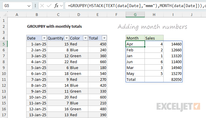
GROUPBY results with month numbers added as a second column - 4

Notice I’ve also removed the sort order setting, so we are back to an alphabetical sort. The month numbers appear as a second row field, but the table is still being sorted by the left-most row field, which is the month name.

Note: We don’t really want the month numbers in the table, and we’ll get rid of them in a another step below.

Sorting the table by month number

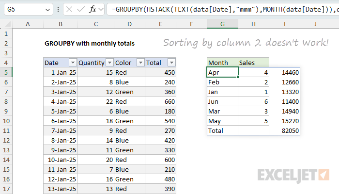
We are now at the point where we can finally sort the table by month number. To do that, we need to specify the column to sort by as an index number. Because we’ve added a column, we need to sort by column 2, the month number. We can do that by adding a sort_order argument to the GROUPBY function like this:

=GROUPBY(HSTACK(TEXT(data[Date],"mmm"),MONTH(data[Date])),data[Total],SUM,,,2)

Unfortunately, this doesn’t work. Why? The problem is that GROUPBY uses a hierarchical relationship between row fields by default. This means the month names override the month numbers, because they appear first in the table:

GROUPBY results where sorting by month number column doesn't work due to hierarchical relationship - 5

We need a way to unlink the month names from the month numbers for sorting. We can do that by supplying 1 for the last argument, which is called field_relationship . This tells GROUPBY to use a table relationship instead of a hierarchy relationship:

=GROUPBY(HSTACK(TEXT(data[Date],"mmm"),MONTH(data[Date])),data[Total],SUM,,,2,,1)

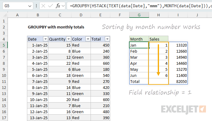
GROUPBY results successfully sorted by month number in chronological order - 6

This works! The month names are no longer overriding the month numbers, and the table is sorted by month number.

Note: you might wonder about adding the month numbers as the first row field instead of the second. This also works. But one consequence is that the word “Total” will be removed from the table when we remove the month number column in the next step. In the end, I decided to keep the month numbers as the second row field because it makes a good example of how the field relationship argument works. See the Alternative formula section below for more details.

Removing the month numbers

The last step in the problem is to remove the month numbers from the table that displays on the worksheet. We still need the month numbers for sorting, so we need to do this outside of the GROUPBY function. The tool we use for this is the CHOOSECOLS function, which is designed to get specific columns from a set of data. In this case, we have three columns total, but we only want to keep columns 1 and 3. Assuming we have a three-column array, we can do that with a generic syntax like this:

=CHOOSECOLS(array,{1,3}) // keep columns 1 and 3

Where array represents the table, and {1,3} is an array of column indices to keep. The final step is to wrap the GROUPBY formula in the CHOOSECOLS function like this:

=CHOOSECOLS(GROUPBY(HSTACK(TEXT(data[Date],"mmm"),MONTH(data[Date])),data[Total],SUM,,,2,,1),{1,3})

You can see the final result in the worksheet below:

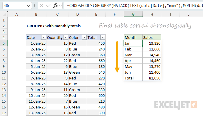
GROUPBY results with months in chronological order and month numbers removed using CHOOSECOLS - 7

We now have data grouped by month with the month names in chronological order.

Summary of steps

Here’s a quick recap of the steps we took:

Started with a basic GROUPBY using TEXT(data[Date],“mmm”) to create month names from the dates. Works fine, but the sort order is alphabetical (Apr, Feb, Jan…) instead of chronological.
Tried reversing the sort with sort_order = -1 but that just flipped the alphabetical order backwards, which still wasn’t what we wanted.
Added month numbers using the HSTACK function because we needed actual numbers (1-12) to sort chronologically.
Set sort_order = 2 to sort by the month numbers, but this didn’t work because GROUPBY was still prioritizing the month names due to its default hierarchical behavior.
Fixed the sorting issue by adding field_relationship = 1 to break the hierarchy and let the month numbers control the sort order.
Used the CHOOSECOLS function to remove the month numbers from the final result since we only need them for sorting, not for display.

Alternative formula #1

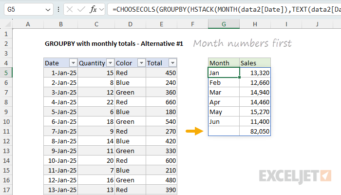
As mentioned above, another way to manage the hierarchy is to reorder the row fields so that the month numbers are the first column:

=CHOOSECOLS(GROUPBY(HSTACK(MONTH(data2[Date]),TEXT(data2[Date],"mmm")),data2[Total],SUM),{2,3})

This formula is a bit simpler because we don’t need to use the field relationship at all. However, one consequence of moving the month numbers to the first column and then using CHOOSECOLS to remove the first column is that the word “Total” is also removed:

Alternative formula #1 with month numbers in the first column and month names in the second column - 8

Alternative formula #2

After I published this article, I got an email from a reader with what I think is an even better idea. It is certainly simpler. The basic idea is to leave all of the dates as dates, but to remap them to the first day of each month. The GROUPBY function still groups the data by month as before. The big advantage is that there is no need to sort manually. Because the dates that represent month names are valid dates, they sort naturally in chronological order. You can see this approach in the worksheet below, where the formula in G5 looks like this:

=GROUPBY(EOMONTH(+data3[Date],-1)+1,data3[Total],SUM)

Inside the GROUPBY function, the EOMONTH function is used to get the first day of the month . The effect is to remap all dates to the first of the month so that GROUPBY can group by month as before. As you can see, this formula is much simpler, but there is one extra step: we need to format the month names with the custom date format “mmm”.

Because of its simplicity, I think this is the best solution to this problem. However, I think the learning process that the rest of the article goes through is valuable, especially because it shows an example of when the field relationship argument is important.

What is that + doing in the EOMONTH formula? Some Excel functions, like EOMONTH , resist spilling when provided a range — they won’t automatically spill results without extra help. Adding an operator like + in front of the range reference forces Excel to evaluate the expression first, which turns the range into an array of values, which EOMONTH can then process. For more details and a list of functions that have this problem, see: Why some functions won’t spill .

Formula for older versions of Excel

The GROUPBY formula only works in the latest version of Excel, which contains dynamic array functions like GROUPBY, HSTACK, and CHOOSECOLS. If you are using an older version of Excel, you will need to use a different approach. I think the easiest approach overall is to enter the month names in column G manually. Then you can use a formula based on SUMPRODUCT in column H to get a monthly total like this:

=SUMPRODUCT(--(TEXT(data2[Date],"mmm")=G5),data2[Total])

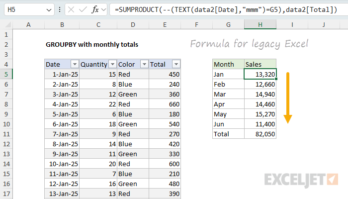
Legacy Excel formula based on SUMPRODUCT function - 10

In this worksheet, data2 is the source data in an Excel Table , and G5 is the abbreviated month name. As the formula is copied down, it will return the total for each month. You will then need to calculate a grand total with the SUM function:

=SUM(H5:H10)

This is a fairly simple approach, but it does require manually entering the month names in column G, and the month names will not dynamically update if the source data changes. For more details on how this formula works, see the SUMPRODUCT function page.

Final thoughts

I’ve been looking for an example where the field relationship argument in the GROUPBY function is needed, and this is a good one. Even after we add the month numbers for sorting, we still can’t sort the months chronologically because of the hierarchy that GROUPBY imposes on row fields. We need to set the field relationship argument to 1 to break the hierarchy and let the month numbers control the sort order. It’s worth noting also that the core GROUPBY formula is quite simple. It’s the process of sorting the months in the correct order that adds complexity.

Explanation

The survey generated almost 3,000 responses, making it a perfect dataset to demonstrate Excel’s new capabilities. In this article, I’ll walk you through using the GROUPBY function to analyze these survey results step by step, showing you how this cool new function can quickly transform raw survey data into useful information.

If you don’t have the new GROUPBY function , a regular Pivot Table would also be an excellent way to analyze these results. In many ways, a Pivot Table is easier, but the trade-off is that a Pivot Table needs to be manually refreshed if data changes, whereas the GROUPBY function will automatically update.

The survey data

The survey data is in an Excel Table called “data” which contains just four columns:

ID – unique numeric ID for each survey response
Version – the Excel version most used by the user
Platform – the platform (Mac or Windows) used
Skill – the self-reported skill level of the user

Core GROUPBY formula

In this example, the goal is to create a table that displays a summary count for each Excel version and the percentage for each count with respect to the total. This is a good job for the GROUPBY function, which is designed to summarize data by grouping rows and aggregating values. As seen in the worksheet below, the core GROUPBY formula looks like this:

=GROUPBY(data[Version],data[Version],COUNTA,0)

For both row_fields and values , we use the Version column. For the function argument, we use COUNTA , since we are counting text values. This gives us a good start. We don’t have a percentage in there yet (or sorting), but we have the correct counts for all versions in the survey data.

Detour

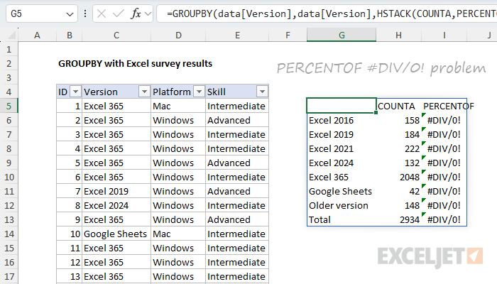
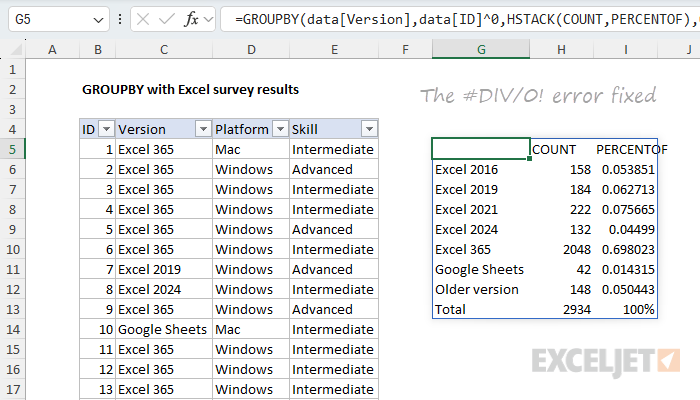
When I set up this formula the first time, my next step was to add the PERCENTOF function to generate a percentage for each count. I also added the HSTACK function so that we have the count and percentage side by side:

=GROUPBY(data[Version],data[Version],HSTACK(COUNTA,PERCENTOF),0)

However, as you can see below, this didn’t work. The COUNT column remained intact, but the PERCENTOF column returned divide-by-zero errors (#DIV/0!).

PERCENTOF divide-by-zero (#DIV/0!) problem - 13

This led to hacky workarounds on my part and then a quick email to the Excel MVP distribution list, where fellow MVP Mark Proctor was kind enough to set me straight. As Mark pointed out, the PERCENTOF function performs a calculation like this:

=SUM(subset)/SUM(totalset)

But it is the GROUPBY function that provides the values for subset and totalset, and this behavior is fixed. Since I was using the actual version data (as text) for values inside the GROUPBY function, I was literally trying to divide a group of text values by another group of text values like this:

=SUM("value","value","value",...)/SUM("value","value","value","value",...)

As you can imagine, this won’t work. We need to adjust our formula to use numeric values so that PERCENTOF can generate meaningful percentages.

I’m leaving this detour in here to emphasize that even people with a lot of Excel experience get into the weeds often and have to backtrack and take a different route. It’s just part of using Excel. 🙃

Back on track with numeric values

To get the PERCENTOF function to work in a case like this, we need to adjust the formula to work with numeric values so that we can calculate a percentage. We don’t need anything fancy. We literally just need a 1 in each row so that we have something to run calculations on. In other words, we want a column of 1s that we can use for values . A column like this isn’t available in the source data, so we’ll need to create it in the formula.

There are a variety of ways to do this in Excel. One approach is to use a function like SEQUENCE or EXPAND to build an array of 1s. Another approach is to use some kind of Boolean operation on an existing array of values. Below are some code snippets that will create a one-column array filled with 1s with the same number of rows as the survey data:

SEQUENCE(ROWS(data),,1,0)
--(data[Version]=data[Version])
--ISNUMBER(data[ID])  
data[ID]^0

In general, I like Boolean operations on source data because they are simple and guarantee we’ll end up with an array of the correct size. Since we already have a numeric value in the ID column, I decided to use the last option, data[ID]^0 , since it’s clever and elegant, and I’m a sucker for that sort of thing. The idea is to raise the numeric IDs to the power of zero, since any number raised to the power of zero equals one. This works nicely in this problem because the numeric ID is part of the source data. Here is the revised formula:

=GROUPBY(data[Version],data[ID]^0,HSTACK(COUNT,PERCENTOF),0)

PERCENTOF divide-by-zero (#DIV/0!) error fixed! - 14

Note that the revised formula provides data[ID]^0 as the values argument. I’ve also switched from COUNTA to COUNT , since we now have numbers to work with. The SUM function would work just as well, since every number is a 1. Whether you use COUNT or SUM is a personal preference. I like COUNT because it intuitively aligns with “counting results” in this example.

You may not have seen the trick of raising numbers to the power of zero to generate an array of ones. I first ran into several years ago while researching formulas created with the obscure but powerful MMULT function . You can try the formula =data[ID]^0 directly on the worksheet to see how it works.

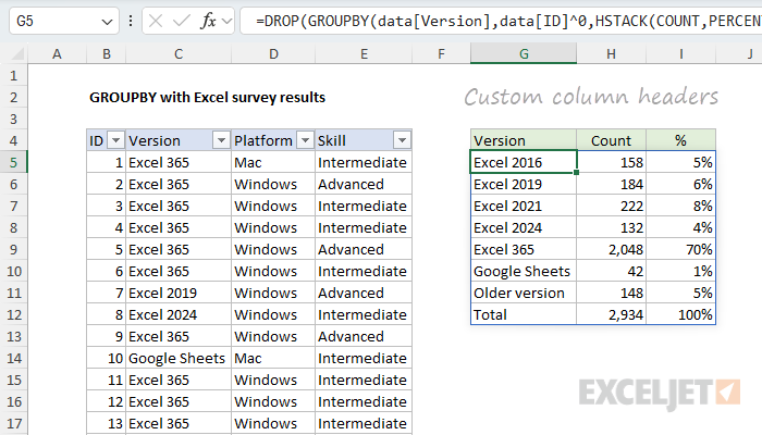
Dropping the function headers

One consequence of adding more than one function with HSTACK is that we get headers above each function, as seen above. The headers appear automatically when you perform more than one calculation with GROUPBY. The headers are useful information in that they quickly tell you what functions are being used, but I like to use my own headers, so I often remove them. W e can easily remove the top header row with the DROP function like this:

=DROP(GROUPBY(data[Version],data[ID]^0,HSTACK(COUNT,PERCENTOF),0),1)

In the worksheet below, I’m using the formula above and have added my own column headers in the row above. After we apply some borders and apply percentage number formatting, the table is almost presentable. However, I really want the Excel versions listed in a specific order, and that means we still have work to do.

GROUPBY formula with custom column headers - 15

It’s worth noting here that you’re on your own when it comes to formatting the output from the GROUPBY function. There are tricks you can use with conditional formatting to auto-format the table, but I’m not using them in this example.

Sorting goal

The main problem at this point is that the version labels are not sorted in any order that makes sense. They are simply sorted alphabetically. I want them to appear in this order:

Excel 365
Excel 2024
Excel 2021
Excel 2019
Excel 2016
Older version
Google Sheets

The GROUPBY function has basic controls for sorting columns and ascending or descending orders, but it doesn’t provide the custom sorting functionality of the SORTBY function . Instead, we’ll need to build the table with GROUPBY, then feed the result into SORTBY. For the actual sorting, we’ll generate an array of sorting values with XMATCH using the order of the list above.

Custom sorting approach

The key feature of Excel’s SORTBY function is that it can sort a range or array using values in another range or array. In other words, if we had an array of numbers that represented the desired sort order, we could use it with SORTBY. Since we already have the Excel versions listed in the desired order on the worksheet in L5:L11, we can generate a custom sorting array with the XMATCH function. The basic idea is to match each version in the GROUPBY table against the sorted list in L5:L11 with the XMATCH function. XMATCH will generate a numeric value for each match, and we’ll use that value for sorting. You can see how this works in the worksheet below, where I’ve configured XMATCH to demonstrate the concept:

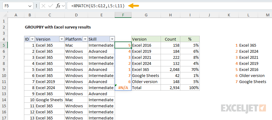
Using XMATCH to create a custom sorting array - 16

Note that “Total” generates an N/A error because it doesn’t appear in our version list. This works fine in this case because the #N/A error automatically sorts to the bottom of the list. The formula above is for illustration only. Below, we move it into the final formula.

Final formula with LET

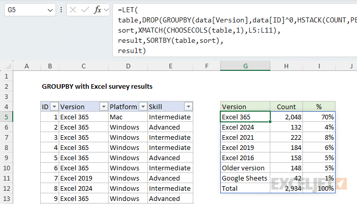
Since we are sorting the table created by GROUPBY after we have dropped the first row, it will be much easier if we use the LET function to keep our formula organized. Here’s the plan: First, we’ll build the basic table and drop the header row, as we did above. Next, we’ll create a custom sort array with XMATCH. Then we’ll feed the table and the custom sort array into the SORTBY function to get a final result. Below is the final formula after implementing LET. Note that we need to use the CHOOSECOLS function to extract just column 1 of the table before we use XMATCH to generate a sorting array:

=LET(
  table,DROP(GROUPBY(data[Version],data[ID]^0,HSTACK(COUNT,PERCENTOF),0),1),
  sort,XMATCH(CHOOSECOLS(table,1), L5:L11),
  result,SORTBY(table, sort),
  result
)

Final GROUPBY formula for analyzing version data - 17

Here is how this formula works:

In the first step, we build the core table with the GROUPBY function and drop the header row. Then we assign the result to the “table” variable.
In the next step, we build a sorting array using the XMATCH function and the list of pre-sorted values in L5:L11. The result is an array of numbers we can use to sort by Excel version in a custom order. We assign this array to the variable “sort”.
Next, we feed the table created in step one and the sort array created in step two into the SORTBY function, and assign the sorted table to “result”.
In the last step, we return the sorted table.

Conclusion

The GROUPBY function offers a powerful and flexible way to summarize survey data dynamically in Excel. It works very well with survey data in the format shown, quickly building the equivalent of a lightweight pivot table. With a few modern functions like HSTACK , PERCENTOF , XMATCH , and SORTBY , we can build a fully automated report that updates instantly when new responses are added. Along the way, we saw how small details, like generating numeric inputs for certain calculations, are an important part of getting this formula to work correctly.

Explanation#

Excel data for source data#

The core GROUPBY formula#

GROUPBY sort options#

Adding the month numbers to sort by#

Sorting the table by month number#

Removing the month numbers#

Summary of steps#

Alternative formula #1#

Alternative formula #2#

Formula for older versions of Excel#

Final thoughts#

Explanation#

The survey data#

Core GROUPBY formula#

Detour#

Back on track with numeric values#

Dropping the function headers#

Sorting goal#

Custom sorting approach#

Final formula with LET#

Conclusion#

Explanation

Excel data for source data

The core GROUPBY formula

GROUPBY sort options

Adding the month numbers to sort by

Sorting the table by month number

Removing the month numbers

Summary of steps

Alternative formula #1

Alternative formula #2

Formula for older versions of Excel

Final thoughts

Explanation

The survey data

Core GROUPBY formula

Detour

Back on track with numeric values

Dropping the function headers

Sorting goal

Custom sorting approach

Final formula with LET

Conclusion