Explanation
The AND function takes multiple arguments and returns TRUE only when all arguments return TRUE. The TODAY function returns the current date. Dates in Excel are simply large serial numbers, so you can create a new relative date by adding or subtracting days. TODAY() + 30 creates a new date 30 days in the future, so when a days is greater than today and less than today + 30, both conditions are true, and the AND function returns true, triggering the rule.
Variable days
Of course, you can adjust days to any value you like:
=AND(B4>TODAY(),B4<=(TODAY()+7)) // next 7 days
=AND(B4>TODAY(),B4<=(TODAY()+45)) // next 45 days
Use other cells for input
You don’t need to hard-code the dates into the rule. To make a more flexible rule, you can use other cells like variables in the formula. For example, you can name cell E2 “days” and rewrite the formula like so:
=AND(B4>TODAY(),B4<=(TODAY()+days))
When you change either date, the conditional formatting rule will respond instantly. By using other cells for input, and naming them as named ranges, you make the conditional formatting interactive and the formula is simpler and easier to read.
Explanation
In this example, the goal is to highlight dates that occur on weekends. In other words, we want to highlight dates that land on either Saturday or Sunday. This problem can be easily solved by applying conditional formatting with a formula based on the WEEKDAY function together with the OR function.
WEEKDAY function
The WEEKDAY function takes a date and returns a number between 1-7 representing the day of week. By default, WEEKDAY returns 1 for Sunday and 7 for Saturday. For example, with the date January 16, 2023 in cell A1, WEEKDAY will return 2, since the day of week is Monday:
=WEEKDAY(A1) // returns 2
OR function
The OR function returns TRUE if any given arguments evaluate to TRUE, and returns FALSE only if all supplied arguments evaluate to FALSE. For example, if cell A1 contains the text “apple”, then:
=OR(A1="pear",A1="apple") // returns TRUE
=OR(A1="pear",A1="orange") // returns FALSE
We can combine the WEEKDAY function with the OR function to test for weekends as explained below.
Test for weekends
To highlight weekends, we need a formula that will return TRUE if a date is either Saturday or Sunday. We can do that by combining the WEEKDAY function with the OR function like this:
=OR(WEEKDAY(C5)=7,WEEKDAY(C5)=1)
Inside the OR function, WEEKDAY returns a number between 1 and 7. If WEEKDAY returns either 7 or 1, the OR function will return TRUE. In all other cases, OR will return FALSE. This is what we need to trigger a conditional formatting rule.
Define the rule
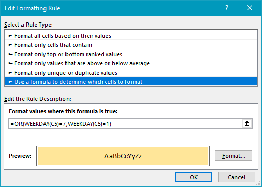
The next step is to define the conditional formatting rule itself. With the range C5:C16 selected, navigate to Home > Conditional Formatting > New rule. Then select “Use a formula to determine which cells to format”. Next, enter the formula above in the formula area and set the desired format. At this point, the conditional formatting rule should look like this:
Highlighting the entire row
The rule above will highlight dates in C5:C16 only. To highlight the entire row when a date is a weekend, start by selecting all data in the range B5:D16. Then use a modified formula that locks the date column:
=OR(WEEKDAY($C5)=7,WEEKDAY($C5)=1)
Note in this version of the formula, $C5 is a mixed reference with the column locked. We do this because we want to make sure that the test for weekend dates is always applied to the dates in column C.
