Explanation
The AND function takes multiple arguments and returns TRUE only when all arguments return TRUE. Dates are just serial numbers in Excel, so earlier dates are always less than later dates. In the above formula, any dates that are greater than or equal to the start date AND less than or equal to the end date will pass both tests and the AND function will return TRUE, triggering the rule.
References to the start and end dates (C2 and E2) are absolute and will not change. References to the date in column C are “mixed” — the column is locked, but the row number is free to change.
Without named ranges
This formula refers to two named ranges: start (C2) and end (E2). Without using named ranges, the formula would look like this:
=AND($C5>=$C$2,$C5<=$E$2)
Embedding dates
This formula exposes the start and end input values directly on the worksheet, so that they can be easily changed. If you want to instead embed (hard-code) the dates directly into the formula, the formula would look like this:
=AND($C5>=DATE(2015,6,1),$C5<=DATE(2015,7,31))
The DATE function ensures that the date is properly recognized. It creates a proper Excel date with given year, month, and day values.
Explanation
In this example, the goal is to highlight rows in the data shown when the date is a specific day of week. The target day of week is a variable selected with a dropdown menu in cell F5, which contains abbreviated day names. This problem can be easily solved by applying conditional formatting with a formula based on the TEXT function. The dropdown menu is implemented with data validation .
TEXT function
The TEXT function returns a number formatted as text, using the number format provided. You can use the TEXT function to convert a valid Excel date into a text value with any standard date formatting. For example, with the date December 1, 2022 in cell A1, the TEXT function will return the following results:
=TEXT(A1,"mmmm") // returns "December"
=TEXT(A1,"dd") // returns "01"
=TEXT(A1,"yyyy") // returns "2022"
=TEXT(A1,"dddd") // returns "Thursday"
=TEXT(A1,"ddd") // returns "Thu"
It is the last example above that we care about in this problem. We can use the abbreviated day name for each date to match against the target date in F5.
Test for day of week
To highlight a specific day of week, we need a formula that will return TRUE when a date lands on the day selected in cell F5. We can do this with the TEXT function like this:
=TEXT(B5,"ddd")=$F$5
The TEXT function extracts an abbreviated day name from the date in B5. When the value returned by TEXT is equal to the target day in cell F5 (which is also abbreviated) the formula will return TRUE. When the result from TEXT is different, the formula will return FALSE. This is what we need to trigger a conditional formatting rule.
Define the rule
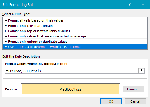
The next step is to define the conditional formatting rule itself. Because we want to highlight entire rows and not just dates, we will apply the rule to all data. With the range B5:C16 selected, navigate to Home > Conditional Formatting > New rule. Then select “Use a formula to determine which cells to format”. Next, enter this formula in the formula area:
=TEXT($B5,"ddd")=$F$5
Then set the desired format, which in this example is a light orange fill. At this point, the conditional formatting rule should look like this:
Note in this version of the formula, $B5 is a mixed reference with the column locked. We do this because we want to make sure that we are always testing just the date value in column B, even as the conditional formatting rule is applied to column C. The row is relative, because it needs to change as the rule is applied to data in different rows. We use an absolute reference for $F$5 because we need that value to remain fixed as the rule is applied to all cells in the data.
