One of the most important operations in Excel formulas is concatenation. In Excel formulas, concatenation is the process of joining one value to another to form a text string . The values being joined can be hardcoded text, cell references, or results from other formulas.
There are two primary ways to concatenate in Excel:
- Manually with the ampersand operator (&)
- Automatically with a function like CONCAT or TEXTJOIN
In the article below, I’ll focus first on manual concatenation with the ampersand operator (&), since this should be your go-to solution for basic concatenation problems. Then I’ll introduce the three Excel functions dedicated to concatenation: CONCATENATE, CONCAT, and TEXTJOIN. These functions can make sense when you need to concatenate many values at the same time. As with so many things in Excel, the most important thing is to understand the basics first.
What is concatenation?
Concatenation is the operation of joining values together to form text. For example, to join “A” and “B” together with concatenation, you can use a formula like this:
="A"&"B" // returns "AB"
The ampersand (&) is Excel’s concatenation operator . Unless you are using one of Excel’s concatenation functions, you will always see the ampersand in a formula that performs concatenation. It’s important to understand that the result from concatenation is always text, even when concatenation involves numbers. For example:
="A"&100 // returns "A100"
=100&200 // returns "100200"
Both of the formulas above return text values, even though some of the values being joined are numeric. In fact, you can transform a number to text by concatenating an empty string ("") to the number like this:
=100&"" // returns "100"
You will sometimes see this technique in a lookup formula that involves numbers and text . Notice in all examples above, text values appear in double quotes (""), while numeric values are not quoted. For example, while 100 is a numeric value, “100” is a text value.
Basic concatenation formula
To explain how concatenation works in a formula in a worksheet, let’s start with a simple example that shows how to concatenate a text string to a value in a cell. With the value 10 in cell B5, this formula will return “Cell B5 contains 10”:

="Cell B5 contains "&B5
There are three things to note in the formula above:
- The text is enclosed in double quotes ("")
- The ampersand joins the text and cell B5
- The cell reference (B5) is not enclosed in quotes
In brief, hardcoded text values are enclosed in double quotes, while cell references, math operators, and function names are not enclosed in quotes.
Now let’s extend the text message above to add a period (.) at the end. In the screen below, the formula in D5 is:

="Cell B5 contains "&B5&"."
In the new formula above, notice two things:
- We need another ampersand (&) to add the period
- The period is text and needs to be enclosed in quotes ("")
Naturally, this is a regular Excel formula that will recalculate automatically. If we change the value in B5 to 15, the new result is “Cell B5 contains 15.”.

This example shows the basics of concatenation in Excel with the ampersand (&) operator. Now let’s look at an example of concatenation with some basic formula logic to customize a message.
Concatenation with conditional logic
There’s nothing special about concatenation, so you can mix in conditional formula logic as needed. In the formula below, we’re using the same basic structure as the example above, with a different message:

="Your score is "&B5&"."
We start the message, concatenate the value from B5, and concatenate the period. Now let’s extend the formula with some conditional logic. Suppose we want to add the text “Nice work!” to the end of the message when the score is 85 or greater. To do this, we can add the IF function like this:
="Your score is "&B5&"."&IF(B5>=85," Nice work!","")
This looks complicated, so let’s break it into parts. Part 1 is the same as before:
="Your score is "&B5&"." // part 1
Part 2 adds conditional logic based on the IF function:
IF(B5>=85," Nice work!","") // part 2
If the score in cell B5 is 85 or higher, IF returns " Nice work!". Otherwise, IF returns an empty string (""). The final formula simply concatenates part 1 to part 2:
="Your score is "&B5&"."&IF(B5>=85," Nice work!","")
Notice we need another ampersand (&) to join part 1 and part 2, since IF is a function name. Also notice that we have included a space (" “) at the start of " Nice work!” so that this text doesn’t run into the period*. The screen below shows how the two formulas compare:
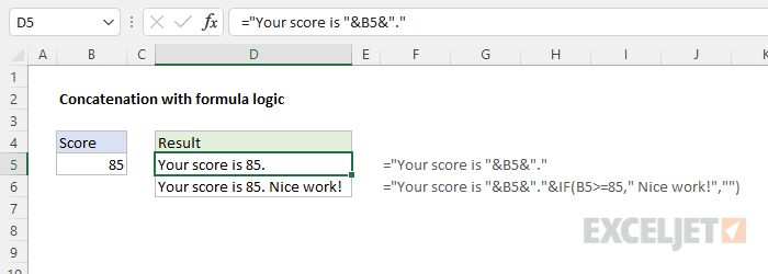
*Note: in more complex formulas that involve concatenation, you will find you frequently need to adjust space or punctuation to keep the message legible.
Concatenation with number formatting
One tricky aspect of concatenation in Excel is number formatting . Number formats in Excel are a powerful way to control the display of numeric values, but they are not part of the number. This means that number formatting will be lost when you concatenate a formatted number. For example, in the worksheet below, B5 contains 99 formatted with the Currency number format. However, when B5 is concatenated in the formula in D5:
="The price is "&B5
the Currency formatting is lost:
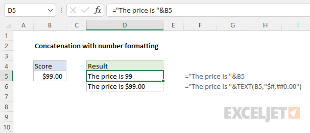
You can add number formatting during concatenation by using the TEXT function in your formula. The formula in D6 is:
="The price is "&TEXT(B5,"$#,##0.00")
In this formula, we place the number in B5 inside the TEXT function and provide a basic Currency number format. As a result, the number 99 is displayed as $99.00 in the result.
Date formatting
Dates are also numbers in Excel and their display is controlled by Date number formatting:
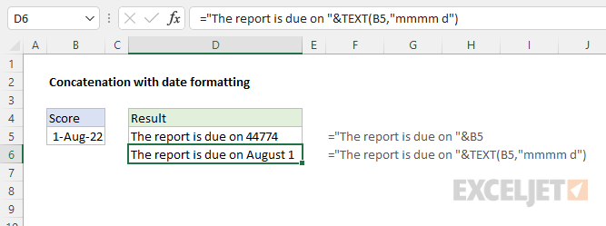
In the worksheet below, the formula in D5 is:
="The report is due on "&B5
Notice the date appears as a raw numeric value . The formula in D5 uses the TEXT function to apply a date format during concatenation:
="The report is due on "&TEXT(B5,"mmmm d")
Excel provides a large number of number formats you can use with the TEXT function. For more details, see Excel custom number formats .
Functions for concatenation
Up to now, we’ve focused on manual concatenation with the ampersand (&) operator. In this section, we’ll look at the functions Excel provides to help with concatenation: CONCATENATE , CONCAT , and TEXTJOIN . In general, CONCATENATE and CONCAT are alternatives to manual concatenation with the ampersand (&) operator, while TEXTJOIN provides more advanced options for working with multiple values. I personally use the ampersand (&) operator as a default approach, and only use the functions below when needed.
CONCATENATE function
The CONCATENATE function is an older function now replaced by the CONCAT function. CONCATENATE allows you to perform simple concatenation only. The values to concatenate and any delimiters are supplied as separate arguments , as seen in the example below:
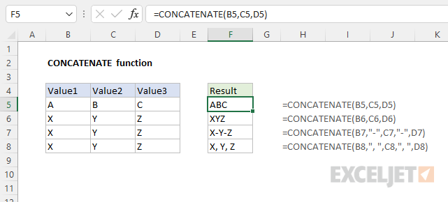
The main benefit of the CONCATENATE function is that values are supplied as separate arguments, with no need for an ampersand (&). The formulas in F5:F8 are:
=CONCATENATE(B5,C5,D5)
=CONCATENATE(B6,C6,D6)
=CONCATENATE(B7,"-",C7,"-",D7)
=CONCATENATE(B8,", ",C8,", ",D8)
Note that hardcoded text values must still be enclosed in double quotes (""), just like manual concatenation with the & operator.
CONCAT function
The CONCAT function replaces the CONCATENATE function in newer versions of Excel. The big difference between the two functions is that CONCAT will accept a range of values:
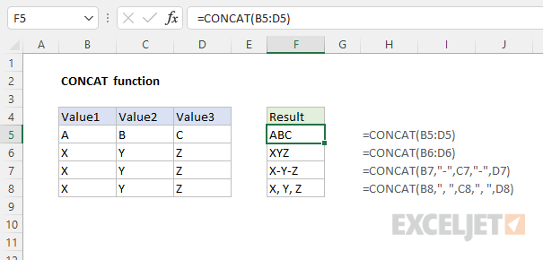
The formulas in F5:F8 are:
=CONCAT(B5:D5)
=CONCAT(B6:D6)
=CONCAT(B7,"-",C7,"-",D7)
=CONCAT(B8,", ",C8,", ",D8)
Notice the first two formulas supply a range directly to CONCAT as a single argument. The ability to provide a range is the primary advantage of CONCAT over CONCATENATE. The next two formulas supply individual values because they are joining values with a delimiter – a hyphen ("-) in the first formula and a comma with a space (", “) in the second formula. Although CONCAT can handle a range, there is no way to provide a delimiter as a separate argument. For this, we need to use the TEXTJOIN function.
TEXTJOIN function
Finally, there is the TEXTJOIN function . Like the CONCAT function, TEXTJOIN is able to accept a range or array of values to concatenate. However, TEXTJOIN provides two additional features that make it especially useful:
- Ability to accept custom delimiter
- Ability to ignore empty values
The syntax for TEXTJOIN is:
=TEXTJOIN (delimiter, ignore_empty, text1, [text2], ...)
The first argument, delimiter , is the delimiter to use when joining values. The second argument, ignore_empty , is a Boolean that indicates whether TEXTJOIN should ignore or process empty values. The remaining arguments, text1 , text2 , etc. represent the values to be joined. The worksheet below shows TEXTJOIN in action:
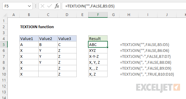
The formulas in F5:F10 are:
=TEXTJOIN("",FALSE,B5:D5)
=TEXTJOIN("",FALSE,B6:D6)
=TEXTJOIN("-",FALSE,B7:D7)
=TEXTJOIN(", ",FALSE,B8:D8)
=TEXTJOIN(", ",FALSE,B9:D9)
=TEXTJOIN(", ",TRUE,B10:D10)
Notice the first two formulas supply an empty string (”") for delimiter , which causes TEXTJOIN to join values directly. The next four formulas all supply one or more characters for delimiter . In cell F9, you can see how the delimiter is repeated when a range contains empty values and ignore_empty is set to FALSE. In F10, ignore_empty has been set to TRUE, and TEXTJOIN ignores the empty value in cell C10.
More examples
Below are more examples that show how concatenation can be used in Excel formulas:
- Join first and last name
- Dynamic worksheet reference
- Count cells greater than
- Make words plural
- Add a line break with a formula
Videos
Here are some videos from our online training that feature concatenation:
- How to join values with the ampersand
- How to use concatenation to clarify assumptions
- Build friendly messages with concatenation
Introduction
What is an array formula anyway?
In simple terms, an array formula is a formula that works with an array of values, rather than a single value. Array formulas can return a single result or multiple results.
That sounds simple enough, and indeed many array formulas are not complex. However, because some array formulas need to be entered in a special way, and some don’t , array formulas live mostly in the geeky realm of super users.
In fact, in the world of Excel formulas, the term “array formula” may be responsible for more confusion than just about any other concept.
With the introduction of Dynamic Arrays in Excel 365 , array formulas are going to become a lot more common, because they are now much easier to use and understand:
- No need for control + shift + enter
- Formulas that return multiple results will spill
Related videos
We’ve been working on a new course, Dynamic Array formulas , and these videos help explain the topics discussed below:
- What is an array formula?
- 3 basic array formula examples
Basic array formula example
In the example below, we want to find the maximum change in temperature over seven days:
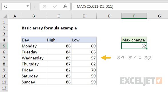
The formula in F5 is:
=MAX(C5:C11-D5:D11)
This is an array formula that returns a single result.
Working from the inside out, we first subtract the low temps from high temps:
C5:C11-D5:D11 // array operation
Each range contains 7 values, which we can expand into arrays like this:
{86;84;89;87;82;85;88}-{69;65;57;62;70;59;59}
This is called an array operation . We are working with multiple values, and the result after subtraction is a new array with 7 values, where each value represents the change in temperature on the given day:
{17;19;32;25;12;26;29} // new array
The new array is returned directly to the MAX function which returns the largest value:
=MAX({17;19;32;25;12;26;29}) // returns 32
You can see that this array formula is actually quite simple!
Traditional Excel - complication and danger
The problem arises when we enter the formula. In “Traditional Excel” (currently, every version of Excel except Office 365), this formula must be entered with control + shift + enter . When entered this way, Excel will display curly braces in the formula bar like this:
{=MAX(C5:C11-D5:D11)}
These curly braces tell you that Excel is handling the formula as an array formula. In other words, Excel is “letting you” work with multiple values.
To most users, that’s pretty strange and confusing. But it gets worse.
If you (or someone else) forget to enter the formula with control + shift + enter, the same exact formula may return an incorrect result.
For example, the formula above without control + shift + enter will return 17, the change in temperature on Monday. This will be a “silent failure” – no warning will occur. The formula will simply stop working correctly.
Obviously, formulas that return incorrect results are bad news :)
Dynamic Excel - simplicity and clarity
The great thing about the Dynamic Array version of Excel , is that array formulas just work . You don’t have to use control + shift + enter with any array formula.
Even better, a formula that returns multiple values will spill these values onto the worksheet. This makes array formulas much easier to understand because it’s obvious when a formula is returning more than one value.
In contrast, the same formulas in previous versions of Excel will display only one result in a single cell, no matter how many values are actually returned.
The bottom line is that working with array formulas in Excel is now easier and more intuitive than ever. You can now use array formulas whenever you like, without worrying about fancy syntax requirements.
Videos
What is an array formula? 3 basic array formulas
