Explanation
The “hashtag” error, a string of hash or pound characters like ####### is not technically an error, but it looks like one. In most cases, it indicates the column width is too narrow to display the value as formatted. You might run into this odd looking result in several situations:
- You apply number formatting (especially dates) to a value
- A cell containing a amount of text in a cell is formatted as a number
- A cell formatted as a date or time contains a negative value
To fix, try increasing the column width first. Drag the column marker to the right until you have doubled or even tripled the width. If the cell displays properly, adjust the width back down as needed, or apply a shorter number format.
If the hash characters persist, even when you make the column much wider, check to see if you have a negative value in the cell, formatted as a date or time. Dates and times must be positive values .
Example
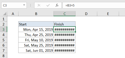
In the worksheet below, Column A contains start dates, and Column B contains a formula that adds 5 days to the start date to get and end date:
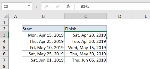
Below, the width of column B has been increased, and dates now display correctly:
Explanation
With the introduction of Dynamic Arrays in Excel formulas , there is more emphasis on arrays . The #CALC! error occurs when a formula runs into a calculation error with an array. The #CALC! error is a “new” error in Excel, introduced with dynamic arrays. It will not appear in older versions of Excel.
Empty array
An empty array can trigger a #CALC! error, and this is the most common reason you may see a #CALC! error in a worksheet, especially when using the FILTER function . This is because FILTER returns a #CALC! error when no values meet criteria – in other words, FILTER returns an empty array .
For example, in the screen below, the FILTER function is set up to filter the source data in B5:D11. However, the formula is asking for all data in the group “x”, which doesn’t exist. The result is a #CALC! error:

=FILTER(B5:D11,B5:B11="x") // no such group, empty array
Fix #1 - adjust filter logic
One option to fix this error is to adjust the filter criteria to return valid results. In the screen below, the formula has adjusted to filter on group “A”, and the formula works normally:
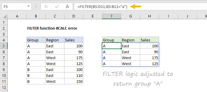
=FILTER(B5:D11,B5:B11="a") // group "a" exists; no empty array
Fix #2 - set is_empty argument
Another option is to provide a “not found” value to return when no results are returned. In the screen below FILTER returns “No results” instead of an error:
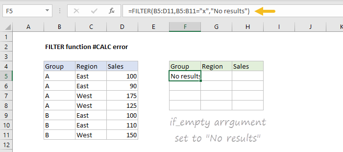
=FILTER(B5:D11,B5:B11="x","No results") // message instead of error
Note: Microsoft documentation mentions other cases that may cause #CALC! errors, notably nested arrays, and unsupported arrays. However, I have not been able to reproduce the error with the examples provided. If you have examples of formulas that throw #CALC! errors, please let me know .
