Explanation
About the #N/A error
The #N/A error appears when something can’t be found or identified. It is often a useful error, because it tells you something important is missing – a product not yet available, an employee name misspelled, a color option that doesn’t exist, etc.
However, #N/A errors can also be caused by extra space characters, misspellings, or an incomplete lookup table. The functions mostly commonly affected by the #N/A error are classic lookup functions, including VLOOKUP , HLOOKUP , LOOKUP , and MATCH .
The best way to prevent #N/A errors is to make sure lookup values and lookup tables are correct and complete. If you see an unexpected #N/A error, check the following first:
- The lookup value is spelled correctly and does not contain extra space characters.
- Values in the lookup table are spelled correctly and do not contain extra space.
- The lookup table is contains all required values.
- The lookup range provided to the function is complete (i.e. does not “clip” data).
- Lookup value type = lookup table type (i.e. both are text, both are numbers, etc.)
- Matching (approximate vs. exact) is set correctly.
Note: if you get an incorrect result, when you should see a #N/A error , make sure you have exact matching configured correctly . Approximate match mode will happily return all kinds of results that are totally incorrect :)
Trapping the #N/A error with IFERROR
One option for trapping the #N/A error is the IFERROR function. IFERROR can gracefully catch any error and return an alternative result .
In the example shown, the #N/A error appears in cell F5 because “ice cream” does not exist in the lookup table, which is the named range “data” (B5:C9).
=VLOOKUP(E5,data,2,0) // "ice cream" is not found
To handle this error, the IFERROR function is wrapped around the VLOOKUP formula like this:
=IFERROR(VLOOKUP(E7,data,2,0),"Not found")
If the VLOOKUP function returns an error, the IFERROR function “catches” that error and returns “Not found”.
Trapping the #N/A error with IFNA
The IFNA function can also trap and handle #N/A errors specifically. The usage syntax is the same as with IFERROR:
=IFERROR(VLOOKUP(A1,table,column,0),"Not found")
=IFNA(VLOOKUP(A1,table,column,0),"Not found")
The advantage of the IFNA function is that it is more surgical, targeting just #N/A errors. The IFERROR function, on the other hand, will catch any error. For example, even if you spell VLOOKUP incorrectly, IFERROR will return “Not found”.
No message
If you don’t want to display any message when you trap an #N/A error (i.e. you want to display a blank cell), you can use an empty string ("") like this:
=IFERROR(VLOOKUP(E7,data,2,0),"")
INDEX and MATCH
The MATCH function also returns #N/A when a value is not found. If you are using INDEX and MATCH together, you can trap the #N/A error in the same way. Based on the example above, the formula in F5 would be:
=IFERROR(INDEX(C5:C9,MATCH(E5,B5:B9,0)),"Not found")
Forcing the #N/A error
If you want to force the #N/A error on a worksheet, you can use the NA function . For example, display #N/A in a cell when A1 equals zero, you can use a formula like this:
=IF(A1=0, NA())
Explanation
The #NAME? error occurs when Excel can’t recognize something. Frequently, the #NAME? occurs when a function name is misspelled, but there are other causes, as explained below. Fixing a #NAME? error is usually just a matter of correcting spelling or a syntax problem. The examples below show misconfigured formulas that return the #NAME error and the steps needed to fix the error and get a working formula again.
Function name misspelled
In the example below, the VLOOKUP function is used to retrieve an item price in F3. The function name “VLOOKUP” is spelled incorrectly, and the formula returns #NAME?
=VLOKUP(E3,B3:C7,2,0) // returns #NAME?

When the formula is fixed, the formula works properly:
=VLOOKUP(E3,B3:C7,2,0) // returns 4.25

Range entered incorrectly
In the example below, the MAX and MIN functions are used to find minimum and maximum temperatures. the formulas in F2 and F3, respectively, are:
=MAX(C3:C7) // returns 74
=MIN(CC:C7) // returns #NAME?

Below the range used in F3 has been fixed:

Note: forgetting to include a colon (:) in a range will also trigger the #NAME? error.
Source data contains #NAME!
If the source data for a function contains a #NAME? error, the calling function might return a #NAME? error. For example, in the worksheet below, the range C3:C7 contains a #NAME? error, so the SUM function also returns #NAME?
=SUM(C3:C7) // returns #NAME?
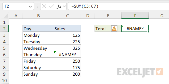
To fix this problem, resolve the errors in the source data.
Named range misspelled
In the example below, the named range “data” equals C3:C7. In F2, “data” is misspelled “daata” and the MAX function returns #NAME?
=MAX(daata) // returns #NAME? error

Below, the spelling is corrected and the MAX function correctly returns 325 as the maximum sales number:
=MAX(data) // returns 325

Notice named ranges are not enclosed by quotes ("") in a formula.
Named range has a local scope
Text value entered without quotes
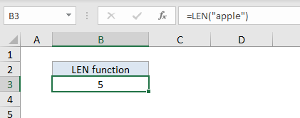
When a text value is input without double quotes, Excel thinks tries to interpret the value as a function name, or named range. This can cause a #NAME? error when no match is found. In the example below, the LEN function is used to get the length of the word “apple”. In B3 the formula is entered without the text string “apple” in quotes (""). Because apple is not a function name or named range, the result is #NAME?
=LEN(apple) // returns #NAME?

Below, quotes have been added and the LEN function now works correctly:
=LEN("apple") // returns 5
Text value with smart quotes
Text values needed to be quoted with straight double quotes (i.e. “apple”). If “smart” (sometimes called “curly”) quotes are used, Excel won’t interpret these as quotes at all and will instead return #NAME?
=LEN(“apple”) // returns #NAME?
To fix this problem, simply replace the smart quotes with straight quotes:
=LEN("apple") // returns 5
Note: some applications, like Microsoft Word, may change straight quotes to smart quotes automatically, so take care if you are moving a formula in and out of different applications or environments.
