Explanation
The #NUM! error occurs in Excel formulas when a calculation can’t be performed. For example, if you try to calculate the square root of a negative number, you’ll see the #NUM! error. The examples below show formulas that return the #NUM error. In general, the fixing the #NUM! error is a matter of adjusting inputs as required to make a calculation possible again.
Example #1 - Number too big or small
Excel has limits on the smallest and largest numbers you can use. If you try to work with numbers outside this range, you will receive the #NUM error. For example, raising 5 to the power of 500 is outside the allowed range:
=5^500 // returns #NUM!
Example #2 - Impossible calculation
The #NUM! error also can appear when a calculation can’t be performed. For example, the screen below shows how to use the SQRT function to calculate the square root of a number. The formula in C3, copied down, is:
=SQRT(B3)
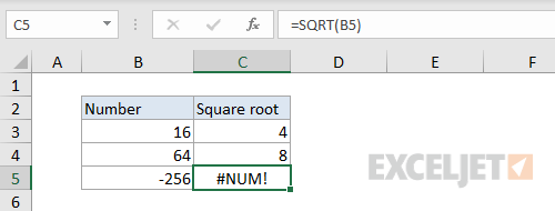
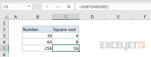
In cell C5, the formula returns #NUM, since the calculation can’t be performed. If you need to get the square root of a negative value (treating the value as positive) you can wrap the number in the ABS function like this:
=SQRT(ABS(B3))
You could also use the IFERROR function to trap the error and return and empty result ("") or a custom message.
Example #3 - incorrect function argument
Sometimes you’ll see the #NUM! error if you supply an invalid input to a function argument . For example, the DATEDIF function returns the difference between two dates in various units. It takes three arguments like this:
=DATEDIF (start_date, end_date, unit)
As long as inputs are valid, DATEDIF returns the time between dates in the unit specified. However, if start date is greater than end date , DATEDIF returns the #NUM error. In the scree below, you can see that the formula works fine until row 5, where the start date is greater than the end date. In D5, the formula returns #NUM.

Notice this is a bit different from the #VALUE! error , which typically occurs when an input value is not the right type. To fix the error shown above, just reverse the dates on row 5.
Example #4 - iteration formula can’t find result
Some Excel functions like IRR , RATE , and XIRR , rely on iteration to find a result. For performance reasons, Excel limits the number of iterations allowed. If no result is found before this limit is reached, the formula returns #NUM error. Iteration behavior can be adjusted at Options > Formulas > Calculation options.
Explanation
About the #REF! error
The #REF! error occurs when a reference is invalid. In many cases, this is because sheets, rows, or columns have been removed, or because a formula with relative references has been copied to a new location where references are invalid. In the example shown, the formula in C10 returns a #REF! error when copied to cell E5:
=SUM(C5:C9) // original C10
=SUM(#REF) // when copied to E5
Preventing #REF errors
The best way to prevent #REF! errors is to prevent then from occurring in the first place. Before you delete columns, rows, or sheets be sure they aren’t referenced by formulas in the workbook. If you are copying and pasting a formula to a new location, you may want to convert some cell references to an absolute reference to prevent changes during the copy operation.
If you cause a #REF! error, it’s best to fix immediately. For example, if you delete a column, and #REF! errors appear, undo that action (you can use the shortcut Control + Z). When you undo, the #REF! errors will disappear. Then edit the formula(s) to exclude the column you want to delete, moving data if needed. Finally, delete the column and confirm there are no #REF! errors.
Clearing multiple #REF! errors
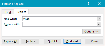
To quickly remove many #REF errors from a worksheet, you can use Find and Replace. Use the shortcut Control + H to open the Find and Replace dialog. Enter #REF! in the find input area, and leave the replace input area blank:
You can then make case-by-case changes with Find next + Replace, or use Replace All to replace all #REF errors in one step.
Fixing #REF errors
#REF errors are somewhat tricky to fix because the original cell reference is gone forever. If you know what the reference should be, you can simply fix it manually. Just edit the formula and replace #REF! with a valid reference. If you don’t know what the cell reference should be, you may have to study the worksheet in more detail before you can repair the formula.
Note: you can’t undo the deletion of a sheet in Excel. If you delete a worksheet tab, and see #REF errors, your best option is probably to close the file and re-open the last saved version. For this reason, always save a workbook (or save a copy) before deleting one or more sheets.
#REF! errors with VLOOKUP
You may see a #REF! error with the VLOOKUP function , when a column is specified incorrectly. In the screen below, VLOOKUP returns #REF! because there is no column 3 in the table range, which is B3:C7:

When the column index is set to the correct value of 2 the #REF! error is resolved and VLOOKUP works properly:

Note: you may also see a #REF error with the INDEX function when a row or column reference is not valid.
Trapping the #REF! error with IFERROR
In most cases, it doesn’t make sense to trap the #REF! error in a formula, because #REF! indicates a low-level problem. However, one situation where IFERROR may make sense to catch a #REF error is when you are building references dynamically with the INDIRECT function .
