Explanation
About spilling and the #SPILL! error
With the introduction of Dynamic Arrays in Excel , formulas that return multiple values " spill " these values directly onto the worksheet. The rectangle that encloses the values is called the " spill range “. When data changes, the spill range will expand or contract as needed. You might see new values added, or existing values disappear.
Video: Spilling and the spill range
Spill behavior is native
It’s important to understand that spill behavior is automatic and native . In Dynamic Excel (Excel 365/2021) any formula , even a simple formula without functions, can spill results. Although there are ways to stop a formula from returning multiple results, spilling itself can’t be disabled with a global setting. Similarly, there is no option in Excel to “disable #SPILL errors. To fix a #SPILL error, you’ll have to investigate and resolve the root cause of the problem.
Spill error information
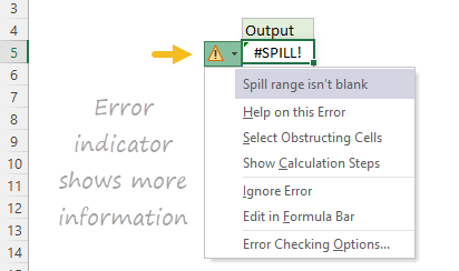
A #SPILL error often occurs when a spill range is blocked by something on the worksheet. Sometimes this is expected. For example, you have entered a formula, expecting it to spill, but existing data in the worksheet is in the way. The solution is just to clear the spill range of any obstructing data. Less often, a #SPILL error has another cause. You can click the spill error indicator to see more information about the cause of the error:
Read below for more information about #SPILL! errors and the specific fixes.
1. Spill range blocked
This is the simplest case to resolve. The formula should return multiple values, but instead it returns #SPILL! because there is already something in the spill range. In the screen below, the “x” is blocking the spill range:

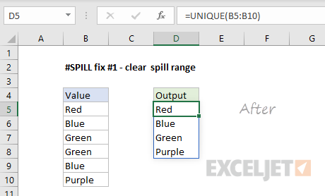
To fix the error, select any cell in the spill range so you can see its boundaries. Then make sure all cells in the spill range are empty. Once the “x” is removed, the UNIQUE function spills results normally:
Cells in the spill range must be empty , so be alert to cells with invisible characters, like spaces.
2. Excel Tables do not support dynamic arrays
Dynamic array formulas are not compatible with Excel tables . If you try to add a dynamic array formula to an Excel Table, the formula will return a #SPILL! error in all rows. The solution in this case is to (1) use an alternative formula or (2) remove the Excel Table by converting it to a normal range with the Convert to Range button on the Table Design tab of the Ribbon: Table Design > Convert to Range
Video: How to remove an Excel Table .
3. Spill range is unknown
Some functions are volatile and can’t be used with dynamic array functions because the result would be “unknown” and dynamic formulas do not currently support arrays of unknown length. For example, the following formula will return a #SPILL! error:
=SEQUENCE(RANDBETWEEN(1,100))
This happens because RANDBETWEEN is volatile and the array returned by SEQUENCE would therefore have an unknown length. The only solution is to avoid dynamic array formulas that create arrays or ranges of an unknown length.
4. Spill range too big
It is possible to write a formula that creates a spill range that extends off the edge of the worksheet. For example, the following formula uses the full column reference A:A:
=A:A+1
If this formula is entered in any row except row 1, it will return a #SPILL! error with a “Spill range is too big” message. This happens because the resulting spill range includes 1,048,576 rows (the limit in Excel) and will run off the bottom of the worksheet. Similarly, the formula below tries to use SEQUENCE to create an array with 17,000 columns:
=SEQUENCE(1,17000)
Because an Excel worksheet contains only 16,384 columns, this formula also returns a #SPILL! error. The solution is to avoid references and formulas that may create spill ranges that do not fit on the worksheet.
5. Implicit intersection (@)
Before Dynamic Arrays , Excel silently applied a behavior called " implicit intersection " to ensure that certain formulas with the potential to return multiple results only returned a single result. In non-dynamic array Excel, these formulas return a normal-looking result with no error. However, in certain cases the same formula entered in Dynamic Excel may create a #SPILL error. For example, in the screen below, cell D5 contains this formula, copied down:
=$B$5:$B$10+3
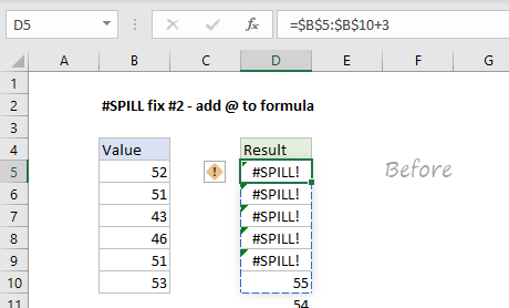
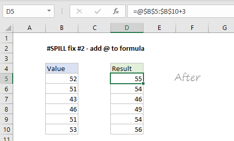
This formula would not throw an error in Excel 2016 because implicit intersection would prevent the formula from returning multiple results. However, in Dynamic Excel, the same formula automatically returns multiple results that crash into each other, since the formula is copied down in D5:D10. One solution is to use the @ character to enable implicit intersection like this:
= @$B$5:$B$10+3
With this change, each formula returns a single result again and the #SPILL error disappears.
Note: this also explains why you might suddenly see the “@” character appear in formulas created in older versions of Excel. This is done to maintain compatibility. Since formulas in older versions of Excel can’t spill into multiple cells, the @ is added to ensure the same behavior when the formula is opened in a version of Excel that supports dynamic arrays.
A better way to fix the #SPILL error above is to use a native dynamic array formula in cell D5:
=B5:B10+3
In Dynamic Excel, this single formula will spill results into the range D5:D10, as seen in the screen below:
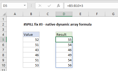
Note there is no need to use an absolute reference since one formula creates all six results.
Explanation
The #VALUE! error appears when a value is not the expected type. This can occur when cells are left blank, when a function expecting a number receives text value, or when dates are evaluated as text by Excel. Fixing a #VALUE! error is usually just a matter of entering the right kind of value.
The #VALUE error is a bit tricky because some functions automatically ignore invalid data. For example, the SUM function just ignores text values, but regular addition or subtraction with the plus (+) or minus (-) operator will return a #VALUE! error if any values are text.
The examples below show formulas that return the #VALUE error, along with options to resolve.
Example #1 - unexpected text value
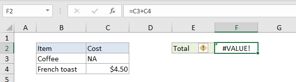
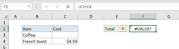
In the example below, cell C3 contains the text “NA”, and F2 returns the #VALUE! error:
=C3+C4 // returns #VALUE!
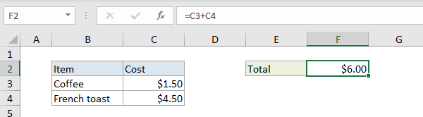
One option to fix is to enter the missing value in C3. The formula in F3 then works correctly:
=C3+C4 // returns 6
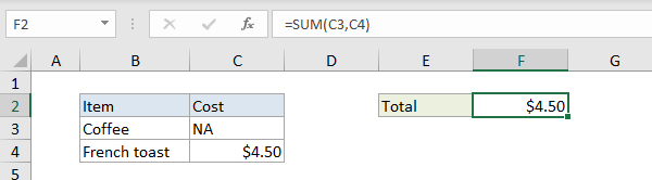
Another option in this case is to switch to the SUM function . The SUM function automatically ignores text values:
=SUM(C3,C4) // returns 4.5
Example #2 - errant space character(s)
Sometimes a cell with one or more errant space characters will throw a #VALUE! error, as seen in the screen below:
Notice C3 looks completely empty. However, if C3 is selected, it is possible to see the cursor sits just a bit to the right of a single space:
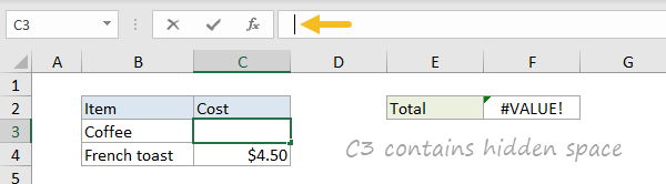
Excel returns the #VALUE! error because a space character is text, so it is actually just another case of Example #1 above. To fix this error, make sure the cell is empty by selecting the cell and pressing the Delete key.
Note: if you have trouble determining whether a cell is truly empty or not, use the ISBLANK function or LEN function to test.
Example #3 - function argument not expected type
The #VALUE! error can also arise when function arguments are not expected types. In the example below, the NETWORKDAYS function is set up to calculate the number of workdays between two dates. In cell C3, “apple” is not a valid date, so the NETWORKDAYS function can’t compute working days and returns the #VALUE! error:

Below, when proper date is entered in C3, the formula works as expected:

Example #4 - dates stored as text
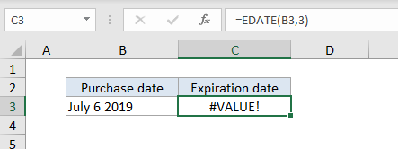
Sometimes a worksheet will contain dates that are invalid because they are stored as text. In the example below, the EDATE function is used to calculate an expiration date three months after a purchase date. The formula in C3 returns the #VALUE! error because the date in B3 is stored as text (i.e. not properly recognized as a date):
=EDATE(B3,3)
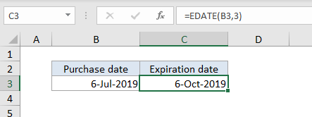
When the date in B3 is fixed, the error is resolved:
If you have to fix many dates stored as text, this page provides some options for fixing.
