Explanation
The #VALUE! error appears when a value is not the expected type. This can occur when cells are left blank, when a function expecting a number receives text value, or when dates are evaluated as text by Excel. Fixing a #VALUE! error is usually just a matter of entering the right kind of value.
The #VALUE error is a bit tricky because some functions automatically ignore invalid data. For example, the SUM function just ignores text values, but regular addition or subtraction with the plus (+) or minus (-) operator will return a #VALUE! error if any values are text.
The examples below show formulas that return the #VALUE error, along with options to resolve.
Example #1 - unexpected text value
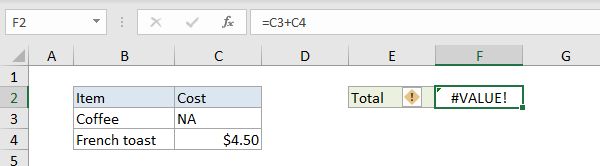
In the example below, cell C3 contains the text “NA”, and F2 returns the #VALUE! error:
=C3+C4 // returns #VALUE!
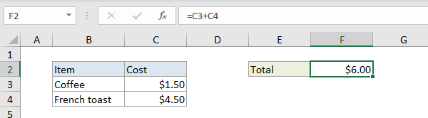
One option to fix is to enter the missing value in C3. The formula in F3 then works correctly:
=C3+C4 // returns 6
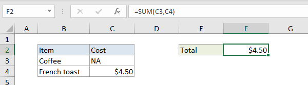
Another option in this case is to switch to the SUM function . The SUM function automatically ignores text values:
=SUM(C3,C4) // returns 4.5
Example #2 - errant space character(s)
Sometimes a cell with one or more errant space characters will throw a #VALUE! error, as seen in the screen below:
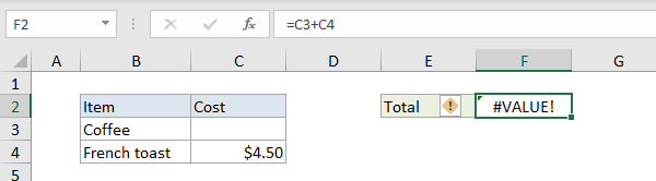
Notice C3 looks completely empty. However, if C3 is selected, it is possible to see the cursor sits just a bit to the right of a single space:
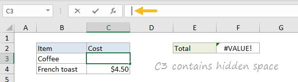
Excel returns the #VALUE! error because a space character is text, so it is actually just another case of Example #1 above. To fix this error, make sure the cell is empty by selecting the cell and pressing the Delete key.
Note: if you have trouble determining whether a cell is truly empty or not, use the ISBLANK function or LEN function to test.
Example #3 - function argument not expected type
The #VALUE! error can also arise when function arguments are not expected types. In the example below, the NETWORKDAYS function is set up to calculate the number of workdays between two dates. In cell C3, “apple” is not a valid date, so the NETWORKDAYS function can’t compute working days and returns the #VALUE! error:

Below, when proper date is entered in C3, the formula works as expected:

Example #4 - dates stored as text
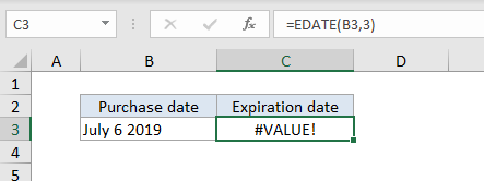
Sometimes a worksheet will contain dates that are invalid because they are stored as text. In the example below, the EDATE function is used to calculate an expiration date three months after a purchase date. The formula in C3 returns the #VALUE! error because the date in B3 is stored as text (i.e. not properly recognized as a date):
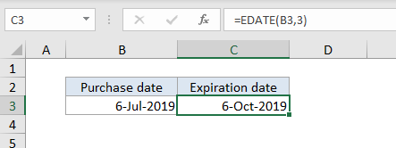
=EDATE(B3,3)
When the date in B3 is fixed, the error is resolved:
If you have to fix many dates stored as text, this page provides some options for fixing.
Explanation
This formula relies on a table with columns for both the full state name and the 2-letter abbreviation. Because we are using VLOOKUP, the full name must be in the first column. For simplicity, the table has been named “states”.
VLOOKUP is configured to get the lookup value from column C. The table array is the named range “states”, the column index is 2, to retrieve the abbreviation from the second column). The final argument, range_lookup, has been set to zero (FALSE) to force an exact match.
=VLOOKUP(C5,states,2,0)
VLOOKUP locates the matching entry in the “states” table, and returns the corresponding 2-letter abbreviation.
Generic mapping
This is a good example of how VLOOKUP can be used to convert values using a lookup table. This same approach can be used to lookup and convert many other types of values. For example, you could use VLOOKUP to map numeric error codes to human readable names.
Reverse lookup
What if you have a state abbreviation, and want to lookup the full state name using the lookup table in the example? In that case, you’ll need to switch to INDEX and MATCH. With a lookup value in A1, this formula will return a full state name with the lookup table as shown:
=INDEX(G5:G55,MATCH(A1,H5:H55,0))
If you want to use the same named range “states” you can use this version to convert a 2-letter abbreviation to a full state name.
=INDEX(INDEX(states,0,1),MATCH(A1,INDEX(states,0,2),0))
Here, we use INDEX to return whole columns by supplying a row number of zero. This is a cool and useful feature of the INDEX function : if you supply zero for row, you get whole column(s) if you supply zero for column, you get whole row(s).
