This article explains in simple terms how to use INDEX and MATCH together to perform lookups. It takes a step-by-step approach, first explaining INDEX, then MATCH, then showing you how to combine the two functions together to create a dynamic two-way lookup. There are more advanced examples further down the page.
- The INDEX Function
- The MATCH function
- INDEX and MATCH together
- Two-way lookup with INDEX and MATCH
- Left lookup with INDEX and MATCH
- INDEX and MATCH with multiple criteria
- Case-sensitive lookup
- Finding the closest match
- INDEX and XMATCH
- More examples
The INDEX Function
The INDEX function in Excel is fantastically flexible and powerful, and you’ll find it in a huge number of Excel formulas, especially advanced formulas. But what does INDEX actually do? In a nutshell, INDEX retrieves the value at a given location in a range. For example, let’s say you have a table of planets in our solar system (see below), and you want to get the name of the 4th planet, Mars, with a formula. You can use INDEX like this:
=INDEX(B3:B11,4)

INDEX returns the value in the 4th row of the range.
Video: How to look things up with INDEX
What if you want to get the diameter of Mars with INDEX? In that case, we can supply both a row number and a column number, and provide a larger range. The INDEX formula below uses the full range of data in B3:D11, with a row number of 4 and column number of 2:
=INDEX(B3:D11,4,2)

INDEX retrieves the value at row 4, column 2.
To summarize, INDEX gets a value at a given location in a range of cells based on numeric position. When the range is one-dimensional, you only need to supply a row number. When the range is two-dimensional, you’ll need to supply both the row and column numbers.
At this point, you may be thinking “So what? How often do you actually know the position of something in a spreadsheet?”
Exactly right. We need a way to locate the position of things we’re looking for.
Enter the MATCH function.
The MATCH function
The MATCH function is designed for one purpose: find the position of an item in a range. For example, we can use MATCH to get the position of the word “peach” in this list of fruits like this:
=MATCH("peach",B3:B9,0)

MATCH returns 3, since “Peach” is the 3rd item. MATCH is not case-sensitive.
MATCH doesn’t care if a range is horizontal or vertical, as you can see below:
=MATCH("peach",C4:I4,0)

Same result with a horizontal range, MATCH returns 3.
Video: How to use MATCH for exact matches
Important: The last argument in the MATCH function is match_type. Match_type is important and controls whether matching is exact or approximate. In many cases, you will want to use zero (0) to force exact match behavior. Match_type defaults to 1, which means approximate match, so it’s important to provide a value. See the MATCH page for more details.
INDEX and MATCH together
Now that we’ve covered the basics of INDEX and MATCH, how do we combine the two functions in a single formula? Consider the data below, a table showing a list of salespeople and monthly sales numbers for three months: January, February, and March.

Let’s say we want to write a formula that returns the sales number for February for a given salesperson. From the discussion above, we know we can give INDEX a row and column number to retrieve a value. For example, to return the February sales number for Frantz, we provide the range C3:E11 with a row 5 and column 2:
=INDEX(C3:E11,5,2) // returns $5194
But we obviously don’t want to hardcode numbers. Instead, we want a dynamic lookup.
How will we do that? The MATCH function of course. MATCH will work perfectly for finding the positions we need. Working one step at a time, let’s leave the column hardcoded as 2 and make the row number dynamic. Here’s the revised formula, with the MATCH function nested inside INDEX in place of 5:
=INDEX(C3:E11,MATCH("Frantz",B3:B11,0),2)
Taking things one step further, we’ll use the value from H2 in MATCH:
=INDEX(C3:E11,MATCH(H2,B3:B11,0),2)

MATCH finds “Frantz” and returns 5 to INDEX for row.
To summarize:
- INDEX needs numeric positions.
- MATCH finds those positions.
- MATCH is nested inside INDEX.
Let’s now tackle the column number.
Two-way lookup with INDEX and MATCH
Above, we used the MATCH function to find the row number dynamically, but we hardcoded the column number. How can we make the formula fully dynamic so we can return sales for any given salesperson in any given month? The trick is to use MATCH twice – once to get a row position, and once to get a column position.
From the examples above, we know MATCH works fine with both horizontal and vertical arrays. That means we can easily find the position of a given month with MATCH. For example, this formula returns the position of March, which is 3:
=MATCH("Mar",C2:E2,0) // returns 3
But of course, we don’t want to hardcode any values , so let’s update the worksheet to allow the input of a month name, and use MATCH to find the column number we need. The screen below shows the result:

A fully dynamic, two-way lookup with INDEX and MATCH.
=INDEX(C3:E11,MATCH(H2,B3:B11,0),MATCH(H3,C2:E2,0))
The first MATCH formula returns 5 to INDEX as the row number, and the second MATCH formula returns 3 to INDEX as the column number. Once MATCH runs, the formula simplifies to:
=INDEX(C3:E11,5,3)
and INDEX correctly returns $10,525, the sales number for Frantz in March.
Note: you could use Data Validation to create dropdown menus to select salesperson and month.
Video: How to do a two-way lookup with INDEX and MATCH
Video: How to debug a formula with F9 (to see MATCH return values)
Left lookup
One of the key advantages of INDEX and MATCH over the VLOOKUP function is the ability to perform a “left lookup”. Simply put, this just means a lookup where the ID column is to the right of the values you want to retrieve, as seen in the example below:
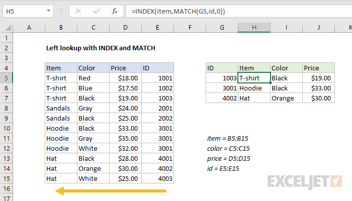
Read a detailed explanation here .
Index and Match with multiple criteria
One of the trickiest problems in Excel is a lookup based on multiple criteria. In other words, a lookup that matches on more than one column at the same time. A nice way to handle these problems is to use Boolean logic , a technique for handling TRUE and FALSE values like 1s and 0s. You can see this approach below, where we are using INDEX and MATCH and Boolean logic to find a price based on three values: Item, Color, and Size:
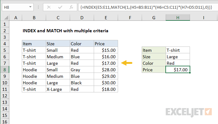
Read a detailed explanation here . You can use this same approach with XLOOKUP .
Note: this is an array formula and must be entered with control + shift + enter in Excel 2019 and older.
For a quick introduction to Booleans in Excel, see these videos from our Dynamic Array Formulas course:
- Introduction to Booleans
- Boolean Algebra in Excel
One benefit of INDEX and MATCH formulas is that they use numeric indexing. This makes it easy to customize behavior to match specific data patterns. For example, you can use a step-based formula to jump directly to relevant data.
Case-sensitive lookup
By itself, the MATCH function is not case-sensitive. However, you use the EXACT function with INDEX and MATCH to perform a lookup that respects upper and lower case, as shown below:
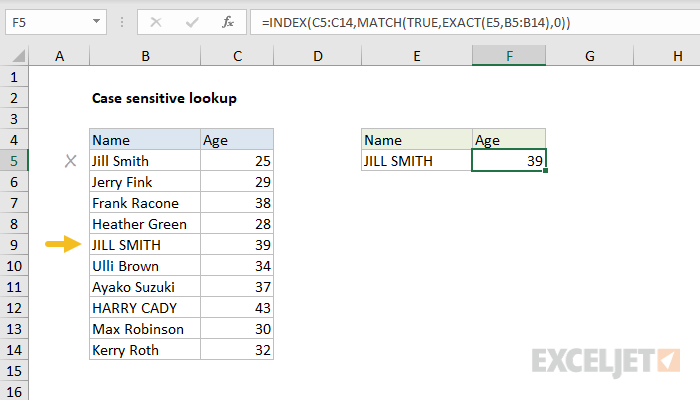
Read a detailed explanation here .
Note: this is an array formula and must be entered with control + shift + enter in Excel 2019 and older.
Closest match
Another example that shows off the flexibility of INDEX and MATCH is the problem of finding the closest match . In the example below, we use the MIN function together with the ABS function to create a lookup value and a lookup array inside the MATCH function. Essentially, we use MATCH to find the smallest difference. Then, we use INDEX to retrieve the associated trip from column B.
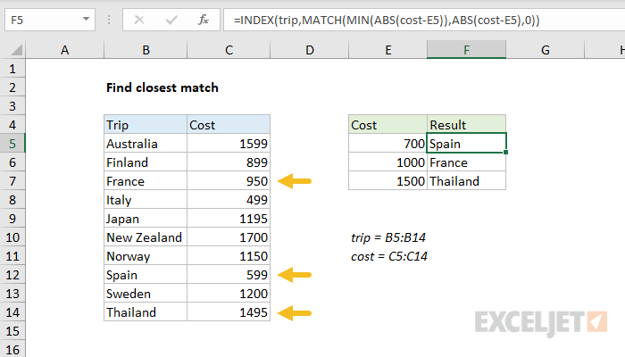
Read a detailed explanation here .
Note: this is an array formula and must be entered with control + shift + enter in Excel 2019 and older.
INDEX and XMATCH
The current version of Excel includes the XMATCH function , which is an upgraded replacement for the MATCH function. Like the MATCH function, XMATCH performs a lookup and returns a numeric position. Also like MATCH, XMATCH can perform lookups in vertical or horizontal ranges, supports both approximate and exact matches, and allows wildcards (* ?) for partial matches. But XMATCH adds even more features. The 5 key differences between XMATCH and MATCH are as follows:
- XMATCH defaults to an exact match, while MATCH defaults to an approximate match.
- XMATCH can find the next larger item or the next smaller item.
- XMATCH can perform a reverse search (i.e. search from last to first).
- XMATCH does not require values to be sorted when performing an approximate match.
- XMATCH can perform a binary search, which is specifically optimized for speed.
- XMATCH can perform a regex match, a powerful way to match complex text patterns.
So, can you simply use XMATCH in an INDEX and MATCH formula instead of MATCH? Yes, absolutely. Using XMATCH instead of the MATCH function “upgrades” the formula to include the benefits listed above.
Using XMATCH instead of the MATCH function “upgrades” the formula to include the benefits listed above.
Replacing MATCH with XMATCH
For exact-match problems, XMATCH is a drop-in replacement for the MATCH function. You can simply change “MATCH” to “XMATCH” as shown below:
=MATCH(value,array,0) // exact match
=XMATCH(value,array,0) // exact match
Note: since XMATCH defaults to an exact match, the zero above is not required. However, when converting MATCH in exact-match mode to XMATCH, you can leave the zero if you like.
For approximate matches, XMATCH behavior is different when match_type is set to 1:
=MATCH(value,array,1) // exact match or next smallest
=XMATCH(value,array,1) // exact match or next *largest*
In addition, XMATCH allows -1 for match type, which is not available with MATCH:
=XMATCH(value,array,-1) // exact match or next smallest
Note: the MATCH function does not offer the search mode argument at all.
XMATCH can also be configured to perform a reverse search and a binary search. For a full description of all of the options available with XMATCH, see this page .
More examples of INDEX + MATCH
Here are some more basic examples of INDEX and MATCH in action, each with a detailed explanation:
- Basic INDEX and MATCH exact (features Toy Story)
- Basic INDEX and MATCH approximate (grades)
- Two-way lookup with INDEX and MATCH (approximate match)
Introduction
Number formats control how numbers are displayed in Excel. The key benefit of number formats is that they change how a number looks without changing any data. They are a great way to save time in Excel because they perform a huge amount of formatting automatically. As a bonus, they make worksheets look more consistent and professional.
Video: What is a number format
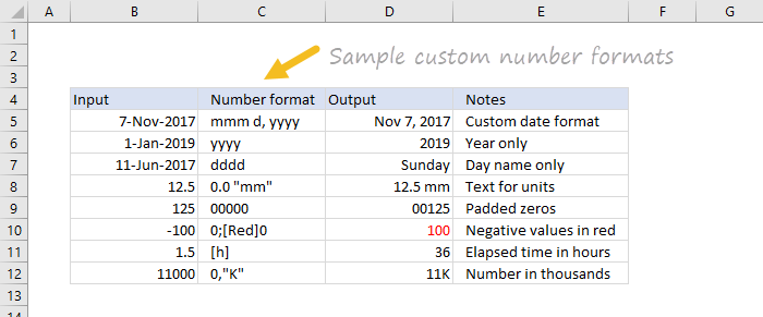
What can you do with custom number formats?
Custom number formats can control the display of numbers, dates, times, fractions, percentages, and other numeric values. Using custom formats, you can do things like format dates to show month names only, format large numbers in millions or thousands, and display negative numbers in red.
Where can you use custom number formats?
Many areas in Excel support number formats. You can use them in tables, charts, pivot tables, formulas, and directly on the worksheet.
- Worksheet - format cells dialog
- Pivot Tables - via value field settings
- Charts - data labels and axis options
- Formulas - via the TEXT function
What is a number format?
A number format is a special code to control how a value is displayed in Excel. For example, the table below shows 7 different number formats applied to the same date, January 1, 2019:
| Input | Code | Result |
|---|---|---|
| 1-Jan-2019 | yyyy | 2019 |
| 1-Jan-2019 | yy | 19 |
| 1-Jan-2019 | mmm | Jan |
| 1-Jan-2019 | mmmm | January |
| 1-Jan-2019 | d | 1 |
| 1-Jan-2019 | ddd | Tue |
| 1-Jan-2019 | dddd | Tuesday |
The key thing to understand is that number formats change the way numeric values are displayed , but they do not change the actual values.
Where can you find number formats?
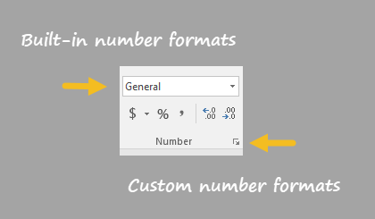
On the home tab of the ribbon, you’ll find a menu of built-in number formats. Below this menu to the right, there is a small button to access all number formats, including custom formats:
This button opens the Format Cells dialog box. You’ll find a complete list of number formats, organized by category, on the Number tab:
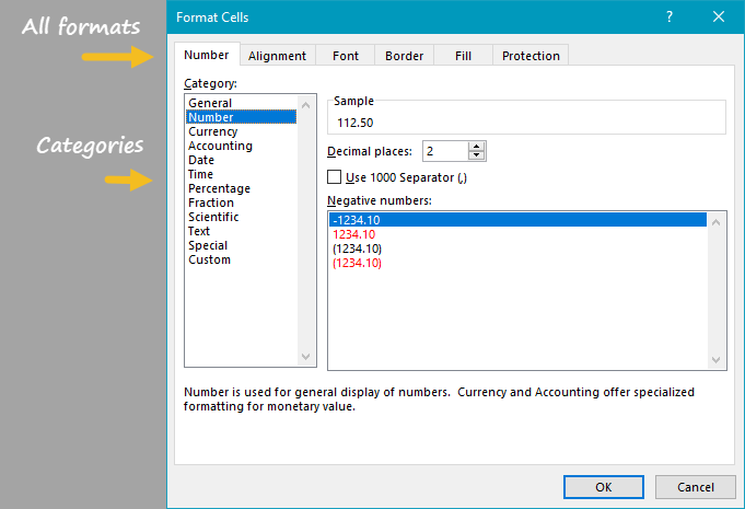
Note: you can open Format Cells dialog box with the keyboard shortcut Control + 1.
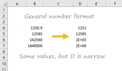
General is default
By default, cells start with the General format applied. The display of numbers using the General number format is somewhat “fluid”. Excel will display as many decimal places as space allows, and will round decimals and use scientific number format when space is limited. The screen below shows the same values in columns B and D, but D is narrower and Excel makes adjustments on the fly.
How to change number formats
You can select standard number formats (General, Number, Currency, Accounting, Short Date, Long Date, Time, Percentage, Fraction, Scientific, Text) on the home tab of the ribbon using the Number Format menu.
Note: As you enter data, Excel will sometimes change number formats automatically. For example, if you enter a valid date, Excel will change to “Date” format. If you enter a percentage like 5%, Excel will change to Percentage, and so on.
Shortcuts for number formats
Excel provides a number of keyboard shortcuts for some common formats:
| Format | Shortcut |
|---|---|
| General format | Ctrl Shift ~ |
| Currency format | Ctrl Shift $ |
| Percentage format | Ctrl Shift % |
| Scientific format | Ctrl Shift ^ |
| Date format | Ctrl Shift # |
| Time format | Ctrl Shift @ |
| Custom formats | Control + 1 |
Where to enter custom formats
At the bottom of the predefined formats, you’ll see a category called custom. The Custom category shows a list of codes you can use for custom number formats, along with an input area to enter codes manually in various combinations.
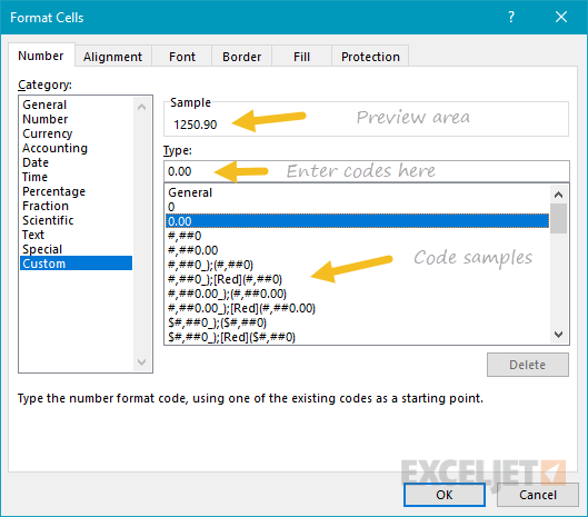
When you select a code from the list, you’ll see it appear in the Type input box. Here you can modify existing custom code, or to enter your own codes from scratch. Excel will show a small preview of the code applied to the first selected value above the input area.
Note: Custom number formats live in a workbook, not in Excel generally. If you copy a value formatted with a custom format from one workbook to another, the custom number format will be transferred into the workbook along with the value.
How to create a custom number format
To create a custom number format follow this simple 4-step process:
- Select cell(s) with values you want to format
- Control + 1 > Numbers > Custom
- Enter codes and watch preview area to see result
- Press OK to save and apply
Tip: if you want base your custom format on an existing format, first apply the base format, then click the “Custom” category and edit codes as you like.
How to edit a custom number format
You can’t really edit a custom number format per se. When you change an existing custom number format, a new format is created and will appear in the list in the Custom category. You can use the Delete button to delete custom formats you no longer need.
Warning: there is no “undo” after deleting a custom number format!
Structure and Reference
Excel custom number formats have a specific structure. Each number format can have up to four sections, separated by semi-colons as follows:
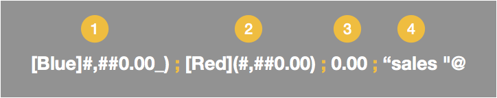
This structure can make custom number formats look overwhelmingly complex. To read a custom number format, learn to spot the semi-colons and mentally parse the code into these sections:
- Positive values
- Negative values
- Zero values
- Text values
Not all sections required
Although a number format can include up to four sections, only one section is required. By default, the first section applies to positive numbers, the second section applies to negative numbers, the third section applies to zero values, and the fourth section applies to text.
- When only one format is provided, Excel will use that format for all values.
- If you provide a number format with just two sections, the first section is used for positive numbers and zeros, and the second section is used for negative numbers.
- To skip a section, include a semi-colon in the proper location, but don’t specify a format code.
Characters that display natively
Some characters appear normally in a number format, while others require special handling. The following characters can be used without any special handling:
| Character | Comment |
|---|---|
| $ | Dollar |
| +- | Plus, minus |
| () | Parentheses |
| {} | Curly braces |
| <> | Less than, greater than |
| = | Equal |
| : | Colon* |
| ^ | Caret |
| ' | Apostrophe |
| / | Forward slash* |
| ! | Exclamation point |
| & | Ampersand |
| ~ | Tilde |
| Space character |
- Update December 2023: The colon (:) and forward slash (/) used to display natively but now must be escaped.
Escaping characters
Some characters won’t work correctly in a custom number format without being escaped. For example, the asterisk (*), hash (#), and percent (%) characters can’t be used directly in a custom number format – they won’t appear in the result. The escape character in custom number formats is the backslash (). By placing the backslash before the character, you can use them in custom number formats:
| Value | Code | Result |
|---|---|---|
| 100 | #0 | #100 |
| 100 | *0 | *100 |
| 100 | %0 | %100 |
Placeholders
Certain characters have a special meaning in custom number format codes. The following characters are key building blocks:
| Character | Purpose |
|---|---|
| 0 | Display insignificant zeros |
| # | Display significant digits |
| ? | Display aligned decimals |
| . | Decimal point |
| , | Thousands separator |
| * | Repeat the following character |
| _ | Add space |
| @ | Placeholder for text |
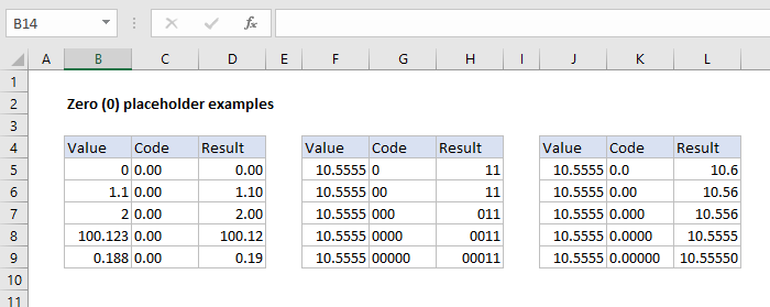
Zero (0) is used to force the display of insignificant zeros when a number has fewer digits than zeros in the format. For example, the custom format 0.00 will display zero as 0.00, 1.1 as 1.10 and .5 as 0.50.
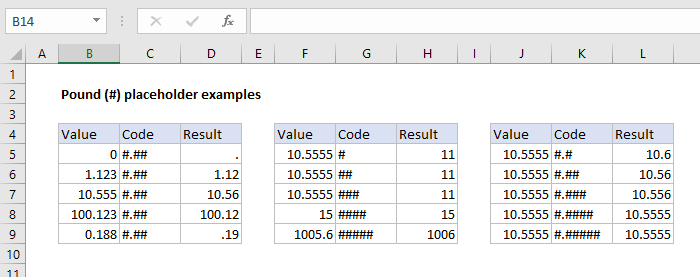
Pound sign (#) is a placeholder for optional digits. When a number has fewer digits than # symbols in the format, nothing will be displayed. For example, the custom format #.## will display 1.15 as 1.15 and 1.1 as 1.1.
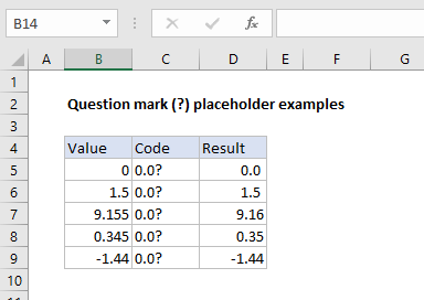
Question mark (?) is used to align digits. When a question mark occupies a place not needed in a number, a space will be added to maintain visual alignment.
Period (.) is a placeholder for the decimal point in a number. When a period is used in a custom number format, it will always be displayed, regardless of whether the number contains decimal values.
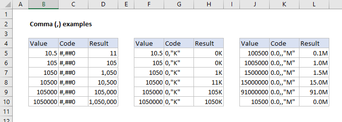
Comma (,) is a placeholder for the thousands separators in the number being displayed. It can be used to define the behavior of digits in relation to the thousands or millions digits.
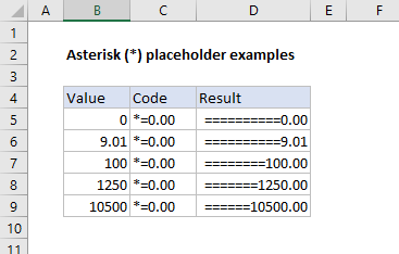
Asterisk (*) is used to repeat characters. The character immediately following an asterisk will be repeated to fill the remaining space in a cell.
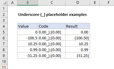
Underscore () is used to add space in a number format. The character immediately following an underscore character controls how much space to add. A common use of the underscore character is to add space to align positive and negative values when a number format is adding parentheses to negative numbers only. For example, the number format “0);(0)” adds a bit of space to the right of positive numbers so that they stay aligned with negative numbers, which are enclosed in parentheses.
At (@) - placeholder for text. For example, the following number format will display text values in blue:
0;0;0;[Blue]@
See below for more information about using color.
Automatic rounding
It’s important to understand that Excel will perform “visual rounding” with all custom number formats. When a number has more digits than placeholders on the right side of the decimal point, the number is rounded to the number of placeholders. When a number has more digits than placeholders on the left side of the decimal point, extra digits are displayed. This is a visual effect only; actual values are not modified.
Number formats for TEXT
To display text together with numbers, enclose the text in double quotes (""). You can use this approach to append or prepend text strings in a custom number format, as shown in the table below.
| Value | Code | Result |
|---|---|---|
| 10 | General" units" | 10 units |
| 10 | 0.0" units" | 10.0 units |
| 5.5 | 0.0" feet" | 5.5 feet |
| 30000 | 0" feet" | 30000 feet |
| 95.2 | “Score: “0.0 | Score: 95.2 |
| 1-Jun | “Date: “mmmm d | Date: June 1 |
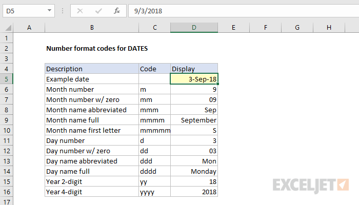
Number formats for DATES
Dates in Excel are just numbers, so you can use custom number formats to change how they are displayed. Excel has many specific codes you can use to display components of a date in different ways. The screen below shows how Excel displays the date in D5, September 3, 2018, with a variety of custom number formats:
Number formats for TIME
Times in Excel are fractional parts of a day. For example, 12:00 PM is 0.5, and 6:00 PM is 0.75. You can use the following codes in custom time formats to display components of a time in different ways. The screen below shows how Excel displays the time in D5, 9:35:07 AM, with a variety of custom number formats:
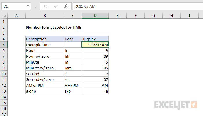
Note: m and mm can’t be used alone in a custom number format since they conflict with the month number code in date format codes.
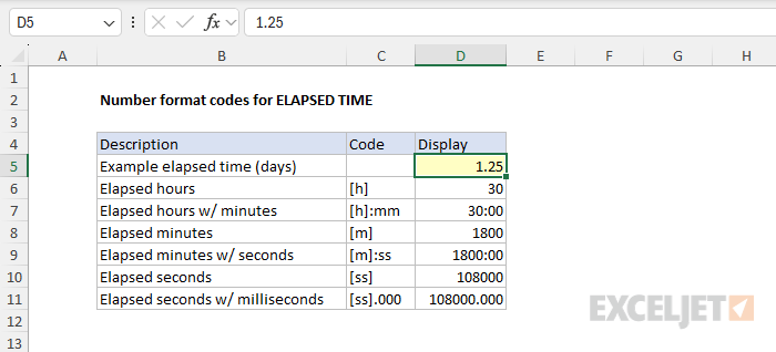
Number formats for ELAPSED TIME
Elapsed time is a special case and needs special handling. By using square brackets, Excel provides a special way to display elapsed hours, minutes, and seconds. The following screen shows how Excel displays elapsed time based on the value in D5, which represents 1.25 days:
Number formats for factional seconds
The following custom number formats will display tenths, hundredths, or thousandths of a second:
mm:ss.0 // tenths of a second (deciseconds)
mm:ss.00 // hundredths of a second (centiseconds)
mm:ss.000 // thousandths of a second (milliseconds)
For a full write-up on working with fractional seconds in Excel, see this article .
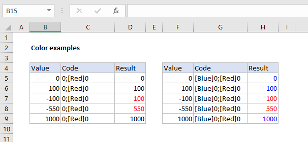
Number formats for COLORS
Excel provides basic support for colors in custom number formats. The following 8 colors can be specified by name in a number format: [black] [white] [red][green] [blue] [yellow] [magenta] [cyan]. Color names must appear in brackets.
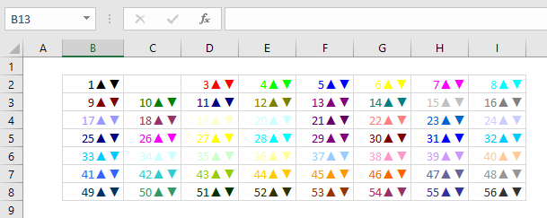
Colors by index
In addition to color names, it’s also possible to specify colors by an index number (Color1, Color2, Color3, etc.) The examples below are using the custom number format: [ColorX]0”▲▼”, where X is a number between 1-56:
[Color1]0"▲▼" // black
[Color2]0"▲▼" // white
[Color3]0"▲▼" // red
[Color4]0"▲▼" // green
etc.
You may need to adjust the name “Color” for other regions or locales. For example, use [ColourX] instead of [ColorX] on a system using British English.
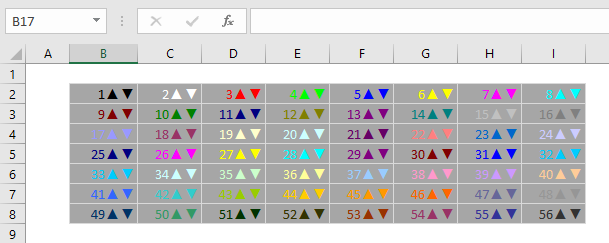
The triangle symbols have been added only to make the colors easier to see. The first image shows all 56 colors on a standard white background. The second image shows the same colors on a gray background. Note the first 8 colors shown correspond to the named color list above.
Apply number formats in a formula
Although most number formats are applied directly to cells in a worksheet, you can also apply number formats inside a formula with the TEXT function . For example, with a valid date in A1, the following formula will display the month name only:
=TEXT(A1,"mmmm")
The result of the TEXT function is always text, so you are free to concatenate the result of TEXT to other strings:
="The contract expires in "&TEXT(A1,"mmmm")
The screen below shows the number formats in column C being applied to numbers in column B using the TEXT function:
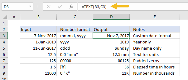
One quirk of the TEXT function relates to double quotes (””) that are part of certain custom number formats. Because the format_text is entered as a text string, Excel won’t allow you to enter the formula without removing the quotes or adding more quotes. For example, to display a large number in thousands, you can use a custom number format like this:
0, "k"
Notice that k appears in quotes (“k”). To apply the same format with the TEXT function, you can use:
=TEXT(A1,"0, k")
Notice the k is not surrounded by quotes. Alternately, you can add extra double quotes as below, which returns the same result:
=TEXT(A1,"0,""K""")
This behavior only occurs when you are hardcoding a format inside TEXT. If you are applying a format entered elsewhere on the worksheet (as in cells C6 and C9 in the worksheet above) you can use a standard number format.
Measurements
You can use a custom number format to display numbers with an inches mark (") or a feet mark (’). In the screen below, the number formats used for inches and feet are:
0.00 \' // feet
0.00 \" // inches

These results are simplistic, and can’t be combined in a single number format. You can however use a formula to display feet together with inches.
Conditionals
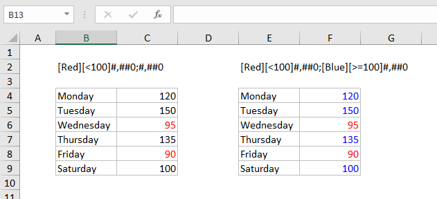
Custom number formats can apply up to two conditions, which are written in square brackets like [>100] or [<=100]. When you use conditionals in custom number formats, you override the standard [positive];[negative];[zero];[text] structure. For example, to display values below 100 in red, you can use:
[Red][<100]0;0
To display values greater than or equal to 100 in blue, you can extend the format like this:
[Red][<100]0;[Blue][>=100]0
To apply more than two conditions, or to change other cell attributes, like fill color, etc. you’ll need to switch to Conditional Formatting , which can apply formatting with much more power and flexibility using formulas.
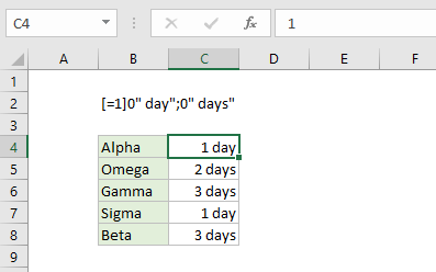
Plural text labels
You can use conditionals to add an “s” to labels greater than zero with a custom format like this:
[=1]0" day";0" days"
Telephone numbers
Custom number formats can also be used for telephone numbers, as shown in the screen below:
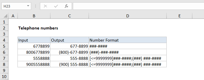
Notice the third and fourth examples use a conditional format to check for numbers that contain an area code. If you have data that contains phone numbers with hard-coded punctuation (parentheses, hyphens, etc.) you will need to clean the telephone numbers first so that they only contain numbers.
Hide all content
You can use a custom number format to hide all content in a cell. The code is simply three semi-colons and nothing else ;;;
To reveal the content again, you can use the keyboard shortcut Control + Shift + ~, which applies the General format.
Other resources
- Developer Bryan Braun built a nice interactive tool for building custom number formats
