How To Use The Mod Function To Repeat Values

Ever use Excel’s MOD function ?

The MOD function performs the modulo operation . It takes a number and a divisor, does the division, and gives you back the remainder.

Unless you’re a programmer, this might seem way too nerdy. Modulo? Seriously? What can the average person do with that?

As it turns out — a lot!

Note: MOD turns up in many compact, elegant formulas in Excel. In fact, if you use MOD in one of your formulas, people will automatically assume you’re an Excel pro, so take care :)

To illustrate how MOD is useful, let me pose a simple problem:

Let’s say you maintain a budget with some monthly expenses, and you’d like to enter an expense that occurs every 3 months, and zero for months in between. You want something like this:

Simple, right? But how to begin…what kind of formula does something every 3 months?

Believe it or not, the MOD function is the key.

Earlier, I mentioned the remainder. The trick in this case is not the remainder itself, but rather what it means when you don’t get a remainder. In other words, when MOD returns zero .

Think about it — when the remainder is zero, it means the divisor goes into the number evenly.

Hmmm…we can use that!

Note: if you want more background on why MOD works well for repeating things, Khan Academy has a nice explanation of modular arithmetic .

We want to do something every 3 months. So, if we run the month number through MOD with a divisor of 3, and get zero as the result, it’s time to add the expense.

Let’s do it.

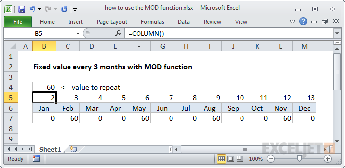
First, let’s add month numbers above our table so we have something to work with right away.

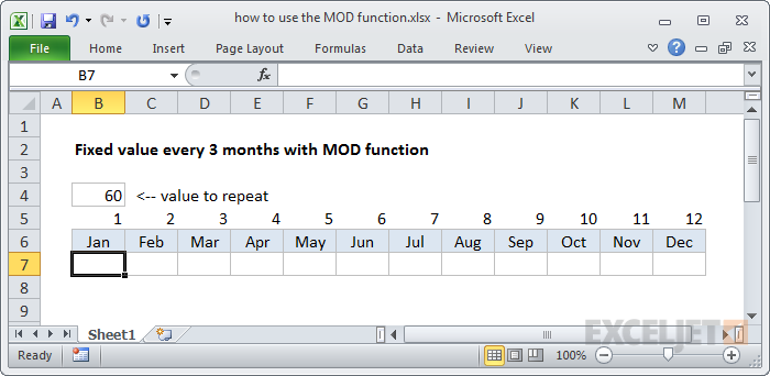
Tip: When you’re building a more complex formula, don’t be afraid to hard-code values that will help you validate your ideas quickly. Think of this as rapid prototyping. Once you know your approach will work, you can come back and figure out how to remove the hard-coded values. Don’t optimize prematurely!

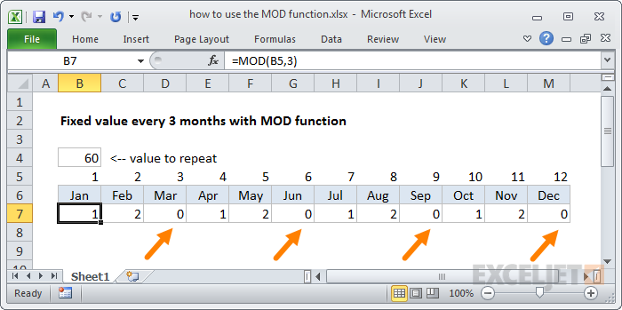
Now, with the month numbers in place, we’ll enter a simple MOD formula.

=MOD(B5,3)

This gives us the remainder in each cell, and every 3 months, we get a remainder of zero.

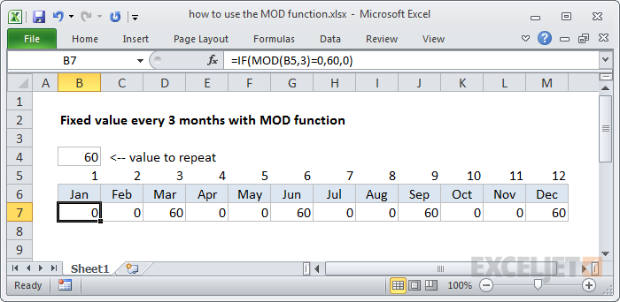
Next, let’s get our value in there when the remainder is zero, and get rid of the other numbers. We can do this by adding an IF statement to test for a zero remainder: if the remainder is zero, return 60, otherwise return 0.

=IF(MOD(B5,3)=0,60,0)

Now we have 60 at every 3rd month and a zero in between. Cool.

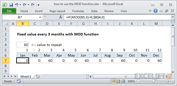
Next, we’ll replace the hardcoded 60 with a reference to B4 so we can easily change it later. Obviously, if the value will never change, there’s no need to do this, but it’s a good practice to expose inputs on the worksheet, especially when they appear in more than one place, and might change later.

We use an absolute reference for B4 so we can copy the formula across without it changing.

=IF(MOD(B5,3)=0,$B$4,0)

This is just what we need, but it’s time to get rid of those unsightly numbers we added above the months.

How can we do it?

There are two ways we can deal with this. One method uses the COLUMN function, and one uses the MONTH function. (See how knowing more Excel functions can be useful?)

We’ll look at COLUMN first…

With the COLUMN function

The COLUMN function returns the column number of a given reference. When you don’t give COLUMN a reference, it returns the column number of the current cell . This is easier to show than explain, so let’s add the COLUMN function to the cells that currently contain month numbers:

This is nice, but notice that it’s not quite what we need. The first number starts with 2, not 1, because the first formula sits in the second column. So this throws off our repeating values.

Easily solved. We just need to subtract 1 from the column number:

COLUMN()-1

Note: think of 1 as an “offset” that you adjust as needed for your situation.

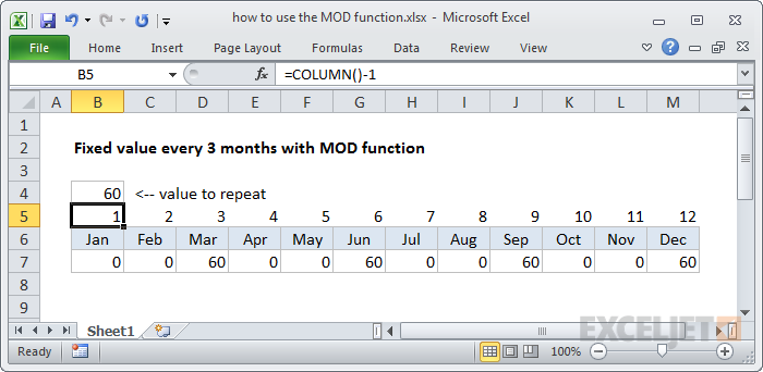
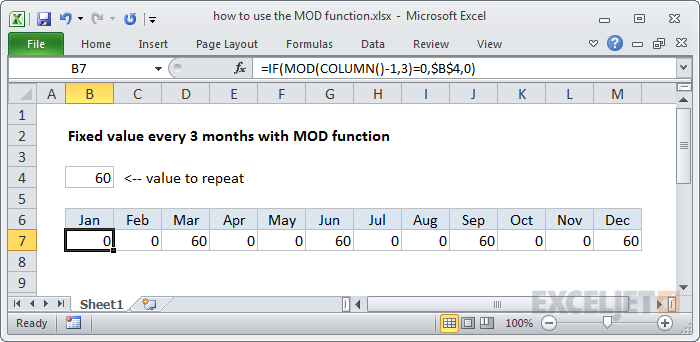
Now COLUMN generates the month numbers we need, and we can update our formula. We simply nest the COLUMN function where we had a reference to the month numbers:

=IF(MOD(COLUMN()-1,3)=0,$B$4,0)

Then we can delete the numbers:

With the MONTH function

While the COLUMN function works fine, it’s a little awkward, because we have to hardcode an offset value to get a correct month number. We only have 12 months — isn’t there some way to use the month numbers directly? Yes, in fact, there is.

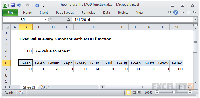
With a little tweak, we can build a more logical formula by using actual dates. To do this, we need to replace the month abbreviations (“Jan”, “Feb”, “Mar”, etc.) with full dates like 1/1/2016, 2/1/2016, 3/1/2016, etc.

Tip: Enter the first two dates then select them both, and use the fill handle to have Excel fill in the rest.

At first, this looks silly — people don’t want to see actual dates for months.

No problem. All we need to do is apply the custom number format “mmm” to the dates, and we’ve got abbreviated month names again:

Same dates with the custom date format “ddd”.

The beauty of this approach is that the column headers now contain regular dates, so we can use normal date functions on them.

And now we can simply use the MONTH function to get the number, and ditch COLUMN:

=IF(MOD(MONTH(B6),3)=0,$B$4,0)

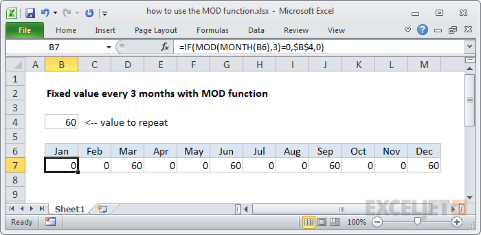
This eliminates that offset value, and the formula will work wherever the budget table appears in the worksheet.

More MOD formulas

As I mentioned, the MOD function is a versatile function and can be used in many ways, so you’ll see it in a variety of formulas. It’s particularly useful for “every nth” type formulas, but it’s handy for other things to. Here’s a list of examples you can use for inspiration.

Sum every nth column Extract time from a date and time Count cells that contain odd numbers Convert time to time zone Highlight integers only Fixed value every N months Highlight every other row Calculate elapsed work time

More Excel formulas and functions

If you want to master more Excel formulas and functions, we have some good resources for you:

1. Excel functions for the minimalist
2. 500 Excel formula examples
3. Excel formula training with practice worksheets

Do you find yourself creating new workbooks in Excel, then making the same changes to every one? Maybe you like to change font size, zoom percent, or the default row height?

If so, you can save yourself time and trouble by setting a default template for Excel to use each time you create a new workbook. As long as you name the template correctly, and put it in the correct location, Excel will use your custom template to create all new workbooks.

The biggest challenge with this tip is figuring out the right location for the template file. This can be maddeningly complex, depending on which platform and version of Excel you use. If you get frustrated and can’t make things work, you can set up your own startup folder manually, as described below.

Settings that can be saved in a template

A template can hold many custom options. Here are a few examples of settings that can be saved in a workbook template:

• Font formatting and styles
• Display options and zoom settings
• Page setup and print options
• Column widths and row heights
• Page formats and print area settings for each sheet
• The number (and type) of sheets in new workbooks
• Placeholder text (titles, column headers, etc.)
• Data validation settings
• Macros, hyperlinks and ActiveX controls
• Workbook calculation options

These settings only apply to new workbooks created after a custom template file is installed.

The process

1. Open a new blank workbook and customize the options as you like
2. Save the workbook as an Excel template with the name " book " (Excel will add .xltx ) *
3. Move the template to the startup folder used by Excel
4. Disable Start screen at General > Start up options) **
5. Quit and relaunch Excel to be sure settings are fresh
6. Test to be sure Excel is using the template when new workbooks are created

• • Not strictly required, but the “New blank workbook” option on the Start screen seems to ignore a custom template (?).

Common startup folder locations

Whenever Excel is launched, it establishes what is called a “startup folder”, which is named XLSTART. The key is to put your template file into this folder so that Excel will find it. Unfortunately, the exact location of XLSTART varies according to the versions of Excel and Windows you use. Here are some common locations:

• C:\Program Files\Microsoft Office\OFFICEx\XLSTART
• C:\Users\user\AppData\Microsoft\Excel\XLSTART
• C:\Users\user\AppData\Roaming\Microsoft\Excel\XLSTART

Can’t find XLSTART?

If you can’t find the startup folder for Excel (XLSTART), you can use the VBA to confirm Excel’s start-up path like this:

1. Run Excel
2. Open the VBA editor (Alt + F11)
3. Open the Immediate Window (Control + G)
4. Type: ? application.StartupPath in the window
5. Press Enter

The startup path will appear below the command. Once you’ve confirmed the location of XLSTART, drop in your template file.

Set your own startup directory

If you can’t find Excel’s startup directory, or if burying your template deep in an application hierarchy just seems wrong, you can tell Excel to look in your own startup folder by setting an option as follows:

1. Create a directory called " xlstart " where you like.
2. Put your custom template in the new directory.
3. At Options > Advanced > General > Open all files in , enter the path to xlstart .
4. Test to make sure the template is working.

Telling Excel about your own startup folder…make sure you use the correct path on your computer!

Test to make sure your template is being used

After you go through the steps to set up a default template, make sure you test to confirm your template is being used. One easy way to do this is to (temporarily) give cell A1 in your template a bright yellow or orange fill. That way, you can immediately see if your custom template is being used when you create a new document. Once you’re sure things are working, remove the marker.

Note 25-Jun-2025 - I had trouble getting Excel to use my custom template on a new Windows 11 machine, even though book.sltx was in the correct location. The problem was Excel using a start screen. If your template is still not loading, check to see if the “Start screen” is enabled at File > Options > General > Startup options. If so, uncheck the option “Show the Start screen when this application starts”. This setting can prevent the template from loading.

Setting a default Excel template on the Mac

The process for setting a default Excel template on a Mac is similar to the steps above for Windows. Again, confirming the startup folder can be tricky, depending on whether you have Excel 2011 or 2016 installed (2008 not tested). In Excel 2016, according to Microsoft, there is currently no startup folder . Also, as of mid-2016, the name of the template should be “workbook” (manually remove the .xltx extension) not “book”.

Because of confusion around the startup folder, here’s what I recommend on a Mac:

1. Create a new directory in your home documents folder called " xlstart “.
2. Go to Preferences > General > At startup, open all files in , and set xlstart as path.
3. Open a new workbook and customize the options as you like
4. Save the workbook as an Excel template with the name " workbook.xltx " inside xlstart .
5. Manually remove the extension " .xltx " so that the file is named only " workbook “.
6. Quit and relaunch Excel to be sure the settings are updated.
7. Test to confirm Excel uses the template when new workbooks are created.

I tested this with Excel 2011 and Excel 2016 installed on the same Mac in May 2016, and both used the same template as expected.

Note: Tested again in January 2020. Step #5 above (removing the extension) was not needed. Also, I was able to use ‘book.xltx’ for the filename, like the Windows version.

Template for new sheets

A workbook template controls the look and layout of sheets already in the workbook, but not new sheets. When you insert a new sheet, it will inherit Excel’s sheet defaults. If you want to control new sheets with your own template, follow the process below.

1. Open a new blank workbook and delete all sheets except one.
2. Make desired customizations to the sheet.
3. Save as an Excel template named " sheet.xltx " to the location determined above. **
4. Close the file.

** If using a non-English version of Excel, you may need to localize this name.

To test that the sheet template is working, open a workbook and add a new sheet. You should see your customizations in all newly inserted sheets.