Explanation
The goal is to do something if a cell contains a given substring. For example, in the worksheet above, a formula returns “x” when a cell contains “abc”. If you are familiar with Excel, you will probably think first of the IF function. However, one limitation of IF is that it does not support wildcards like “?” and “*”. This means we can’t use IF by itself to test for a substring like “abc” that might appear anywhere in a cell. One solution is to create a logical test with the SEARCH and ISNUMBER functions, and then use an IF statement to return a final result. This approach is explained below.
Finding text in a cell
The SEARCH function is designed to look for specific text inside a larger text string. If SEARCH finds the text, it returns the position of the text as a number. If the text is not found, SEARCH returns a #VALUE error. For example, the formulas below show the result of looking for the letters “a”, “p”, “e”, and “z” in the text “apple”:
=SEARCH("a","apple") // returns 1
=SEARCH("p","apple") // returns 2
=SEARCH("e","apple") // returns 5
=SEARCH("z","apple") // returns #VALUE!
Notice that SEARCH returns a numeric position for the first three letters, and returns a #VALUE! error for “z”, which is not found. The screen below shows how the formulas above can be transferred to a workbook. The text to search appears in column B and the character to look for is hard coded into the SEARCH function:

Finding a word in a cell
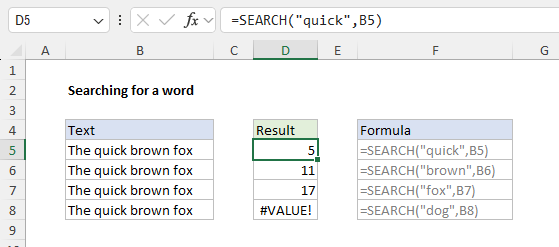
You can use the SEARCH function to find words as well. Notice that SEARCH returns the starting position of the word in the text string:
=SEARCH("quick","The quick brown fox") // returns 5
=SEARCH("brown","The quick brown fox") // returns 11
=SEARCH("fox","The quick brown fox") // returns 17
=SEARCH("dog","The quick brown fox") // returns #VALUE!
As before, if the “find text” isn’t found, SEARCH returns a #VALUE! error as in the last example, where the word “dog” is not found. The screen below shows how the formulas can be set up in a spreadsheet. The text to search is in column B. The word to search for is typed directly into the SEARCH function:
The formulas above work fine. However, we don’t want the position of the text in a cell, what we really want is a TRUE or FALSE result. Enter the ISNUMBER function.
Converting results to TRUE and FALSE
Since our goal is to use an IF statement, we want a logical test that will return TRUE or FALSE. The SEARCH function doesn’t work by itself because it returns either a numeric position or an error. However, we can easily convert the results from SEARCH into TRUE and FALSE values with the ISNUMBER function , which returns TRUE for numeric values and FALSE for anything else:
=ISNUMBER(2) // returns TRUE
=ISNUMBER("a") // returns FALSE
=ISNUMBER(#VALUE!) // returns FALSE
To convert the result from the SEARCH function into a TRUE or FALSE value, we simply place the SEARCH function inside the ISNUMBER function as shown below:
=ISNUMBER(SEARCH("fox","The brown fox")) // returns TRUE
=ISNUMBER(SEARCH("dog","The brown fox")) // returns FALSE
To recap: if SEARCH finds the text in the text string, it returns the position as a number, and ISNUMBER returns TRUE. If SEARCH can’t find the text, it returns an error, and ISNUMBER returns FALSE. We now have what we need to create an IF statement to check if a cell contains text.
If a cell contains a word then
Now that we have a formula that returns TRUE or FALSE, we can use the combination of SEARCH + ISNUMBER as the logical test inside the IF function , and return whatever result we want. In the worksheet shown, we have a list of email addresses, and we want to identify the emails that contain “abc”. The formula in cell C5 looks like this:
=IF(ISNUMBER(SEARCH("abc",B5)),"x","")
The SEARCH function is configured to look for “abc” inside cell B5. If “abc” is found anywhere in cell B5, SEARCH returns a number and ISNUMBER returns TRUE. The IF function then returns “x” as a final result. If “abc” is not found , SEARCH returns an error and ISNUMBER returns FALSE. The IF function then returns an empty string ("") as a final result.
Return matching values
With a small adjustment, we can return the value that contains “abc” instead of returning “x”:
<img loading=“lazy” src=“https://exceljet.net/sites/default/files/images/formulas/inline/if_cell_contains_return_value.png" onerror=“this.onerror=null;this.src=‘https://blogger.googleusercontent.com/img/a/AVvXsEhe7F7TRXHtjiKvHb5vS7DmnxvpHiDyoYyYvm1nHB3Qp2_w3BnM6A2eq4v7FYxCC9bfZt3a9vIMtAYEKUiaDQbHMg-ViyGmRIj39MLp0bGFfgfYw1Dc9q_H-T0wiTm3l0Uq42dETrN9eC8aGJ9_IORZsxST1AcLR7np1koOfcc7tnHa4S8Mwz_xD9d0=s16000';" alt=“If cell contains “abc” return value - 3”>
To return a cell of the value when it contains “abc”, we provide a reference for the value if true argument. If FALSE, we supply an empty string (””) which will display as a blank cell. The formula in cell C5 is:
=IF(ISNUMBER(SEARCH("abc",B5)),B5,"")
If column contains value then
If you need to check a column for a specific text value, the simplest approach is to switch to the COUNTIF function with wildcards. For example, to return “Yes” if column A contains the word “dog” in any cell and “No” if not, you can use a formula like this:
=IF(COUNTIF(A:A,"*dog*"),"Yes","No")
The asterisks (*) are wildcards that match the text “dog” with any number of characters before or after. With this configuration, the COUNTIF function will return a count of cells that contain “dog” anywhere in the cell. If the count is a positive number, the IF function will evaluate the number as TRUE. If no cells contain “dog”, COUNTIF will return zero and the IF function will evaluate this result as FALSE.
Notes
- The SEARCH function is not case-sensitive. If you need a case-sensitive option you can switch to the FIND function as explained here .
- If the goal is to return all matching cells or records together, see the FILTER function .
Explanation
The goal is to do something if a cell contains one substring or another. Most users will think first of the IF function. However, one problem with IF is that it does not support wildcards like “?” and “*”. This means we can’t use IF by itself to test for a substring like “abc” or “xyz” that might appear anywhere in a cell . One option (seen in the example) is to create a logical test with ISNUMBER, SEARCH, and OR, then use the IF function to return a final result. Another approach is to use the COUNTIF function with the SUM function to create the logical test. Both approaches are explained below.
OR + SEARCH + ISNUMBER
The SEARCH function is designed to look inside a text string for a given substring. If SEARCH finds the substring, it returns the position of the substring in the text as a number. If the substring is not found, SEARCH returns a #VALUE error. For example:
=SEARCH("p","apple") // returns 2
=SEARCH("z","apple") // returns #VALUE!
The ISNUMBER function . ISNUMBER returns TRUE for numeric values and FALSE for anything else:
=ISNUMBER(2) // returns TRUE
=ISNUMBER("a") // returns FALSE
We can use ISNUMBER to convert the result from SEARCH into a TRUE or FALSE value like this:
=ISNUMBER(SEARCH("p","apple")) // returns TRUE
=ISNUMBER(SEARCH("z","apple")) // returns FALSE
If SEARCH finds the substring, it returns the position as a number, and ISNUMBER returns TRUE. If SEARCH doesn’t find the substring, it returns an error, and ISNUMBER returns FALSE. This works fine, but the challenge in this problem is that we need to test for two substrings , not one. We can do this by using SEARCH and ISNUMBER twice inside the OR function:
=OR(ISNUMBER(SEARCH("abc",B5)),ISNUMBER(SEARCH("xyz",B5)))
Now if either of the expressions returns TRUE, the OR function will return TRUE and trigger the IF function. One way to simplify the formula a bit is to use an array constant and a single expression like this:
=OR(ISNUMBER(SEARCH({"abc","xyz"},B5)))
An array constant is a structure that holds multiple values. It works like a range in Excel, except the values in an array constant are hard coded. Because we are giving SEARCH two substrings, it will return two results. The ISNUMBER function will also return two results to the OR function, which will evaluate these results as before.
Note: the SEARCH function is not case-sensitive. If you need a case-sensitive option you can switch to the FIND function as explained here .
IF function
Putting this all together, we can use the formula above inside the IF function as the logical test like this:
=IF(OR(ISNUMBER(SEARCH({"abc","xyz"},B5))),"x","")
This is the formula used in cell D5 of the example. As the formula is copied down, it returns “x” if an email address contains either “abc” or “xyz” and an empty string ("") if not. You are free to adjust the IF formula to return whatever values you like.
Note: the IF function simply leaves an “x” in a cell as a marker. I f the goal is to retrieve all matching cells or records, see the FILTER function .
COUNTIF + SUM
Another way to solve this problem is with the COUNTIF function together with the SUM function like this:
=IF(SUM(COUNTIF(B5,{"*abc*","*xyz*"})),"x","")
The core of this formula is COUNTIF, which returns zero if none of the substrings is found, and a positive number if at least one substring is found. The twist is that we are giving COUNTIF more than one substring to look for in the criteria, supplied as an " array constant “. As a result, COUNTIF will return an array of counts, one count per condition. Because we are getting back an array from COUNTIF, we use the SUM function to sum all items in the array. The result goes into the IF function as the logical_test . Any non-zero number will be evaluated as TRUE.
Note that we are also using the asterisk (*) as a wildcard for zero or more characters on either side of the substrings. This is what allows COUNTIF to count the substrings anywhere in the text (i.e. this provides the “contains” behavior).
Notes
- If you are testing many values, you can use a range instead of an array constant to provide values to check. In Excel 2019 and earlier, using a range will make the formula an array formula that must be entered with control + shift + enter. In the current version of Excel, no special handling is required.
- The COUNTIF function will accept ranges only for the range argument; you can’t feed COUNTIF an array that comes from another formula. This can be a problem when working with dynamic array formulas , where it is more common to pass arrays from one formula to another. The OR + SEARCH + ISNUMBER formula does not have this limitation.
