Explanation
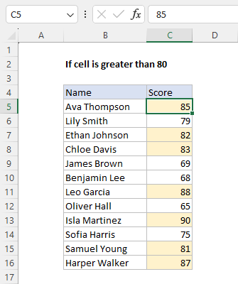
The aim is to mark records with an “x” if a score is greater than 80 and leave the cell blank if the score is less than 80. This can be achieved using the IF function in Excel.
IF function
The IF function runs a logical test and returns one value for a TRUE result, and another value for a FALSE result. The generic syntax for IF looks like this:
=IF(logical_test,if_true,if_false)
The IF function can return a value, a cell reference, or even another formula. In the worksheet shown, the goal is to identify rows where the score is greater than 80 by returning “x” as a marker. To accomplish this task, the formula in cell E5 is:
=IF(C5>80,"x","")
In this formula, the logical test is this expression:
C5>80
This expression returns TRUE if the value in C5 is greater than 80 and FALSE if not. In cell F5, the result is TRUE because C5 contains 85. The IF function then returns “x” as a final result:
=IF(C5>80,"x","") // returns "x"
In cell F6, the expression returns FALSE because C6 contains 79. The IF function returns an empty string "" as a final result:
=IF(C6>80,"x","") // returns ""
In Excel, an empty string ("") displays nothing. The result returned by the IF function can be customized as needed. For example, to return “Yes” if a score is greater than 80 and “No” if not, you can use this formula:
=IF(C5>80,"Yes","No")
Note that if no value is provided for the value_if_false argument, the formula will return FALSE for scores not greater than 80.
Conditional formatting
Another way to identify cells with a value greater than 80 is to use conditional formatting , as seen below:
This is an example of applying conditional formatting with a formula. The formula used to highlight scores greater than 80 is:
=C5>80
The formatting is automatic. If a score is changed to a number greater than 80, the yellow highlighting will appear. You can find more conditional formatting examples here .
Explanation
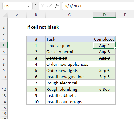
The goal is to create a formula that returns “Done” in column E when a cell in column D is not blank (i.e., contains a value). In the worksheet shown, column D records the date a task is completed. If column D contains a date (i.e. is not empty), we can assume the task is complete. This problem can be solved with the IF function alone or with the IF function and the ISBLANK function. It can also be solved with the LEN function. All three approaches are explained below.
IF function
The IF function runs a logical test and returns one value for a TRUE result, and another value for a FALSE result. Use IF to test for a blank cell like this:
=IF(A1="",TRUE) // IF A1 is blank
=IF(A1<>"",TRUE) // IF A1 is not blank
In the first example, we test if A1 is empty with ="". In the second example, the <> symbol is a logical operator that means “not equal to”, so the expression A1<>"" means A1 is “not empty”. In the worksheet shown, we use the second concept in cell E5 like this:
=IF(D5<>"","Done","")
If D5 is “not empty”, the result is “Done”. If D5 is empty, IF returns an empty string ("") which displays as nothing in Excel. As the formula is copied down, it returns “Done” only for cells in column D that contain a value. To display both “Done” and “Not done”, you can adjust the formula like this:
=IF(D5<>"","Done","Not done")
ISBLANK function
Another way to solve this problem is with the ISBLANK function . The ISBLANK function returns TRUE when a cell is empty and FALSE if not. To use ISBLANK only, you can rewrite the formula like this:
=IF(ISBLANK(D5),"","Done")
Notice the TRUE and FALSE results have been reversed. The logic now is if cell D5 is blank . To maintain the original logic, you can nest ISBLANK inside the NOT function like this:
=IF(NOT(ISBLANK(D5)),"Done","")
The NOT function reverses the output from ISBLANK.
LEN function
One problem with testing for blank cells in Excel is that ISBLANK(A1) or A1="" will return FALSE if A1 contains a formula that returns an empty string. In other words, if a formula returns an empty string in a cell, Excel interprets the cell as “not empty” even though it looks empty. To work around this problem, you can use the LEN function to test for characters in a cell like this:
=IF(LEN(A1)<>0,"Open","")
This is a more literal formula. We are not asking Excel if A1 is blank, we are literally counting the characters in A1. The LEN function will return a non-zero number only when a cell contains actual characters. Using the LEN function this way works for cells containing formulas as well as cells without formulas.
Conditional formatting
Another way to highlight tasks based on a cell that is not blank is to use conditional formatting . In the screen below, this formula is used to highlight rows that do not contain a completion date:
=$D5<>""
This is an example of applying conditional formatting with a formula. When a date is entered in column D, the formatting will be applied. More examples here .
