Explanation
In the example shown, we want to mark or “flag” records where the color is red OR green. In other words, we want to check the color in column B, and then leave a marker (x) if we find the word “red” or “green”. In D6, the formula is:
=IF(OR(B6="red",B6="green"),"x","")
This is an example of nesting – the OR function is nested inside the IF function. Working from the inside out, the logical test is created with the OR function:
OR(B6="red",B6="green") // returns TRUE
OR will return TRUE if the value in B6 is either “red” OR “green”, and FALSE if not. This result is returned directly to the IF function as the logical_test argument. The color in B6 is “red” so OR returns TRUE:
=IF(TRUE,"x","") // returns "x"
With TRUE as the result of the logical test, the IF function returns a final result of “x”.
When the color in column B is not red or green, the OR function will return FALSE, and IF will return an empty string ("") which looks like a blank cell:
=IF(FALSE,"x","") // returns ""
As the formula is copied down the column, the result is either “x” or “”, depending on the colors in column B.
Note: if an empty string ("") is not provided for value_if_false, the formula will return FALSE when the color is not red or green.
Increase price if color is red or green
You can extend this formula to run another calculation, instead of simply returning “x”. For example, let’s say you want to increase the price of red and green items only by 15%. In that case, you can use the formula in column E to calculate a new price:
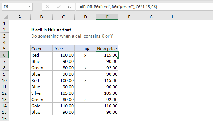
=IF(OR(B6="red",B6="green"),C6*1.15,C6)
The logical test is the same as before. However, the value_if_true argument is now a formula:
C6*1.15 // increase price 15%
When the result of the test is TRUE, we multiply the original price in column C by 1.15, to increase by 15%. If the result of the test is FALSE, we simply return the original price. As the formula is copied down, the result is either the increased price or the original price, depending on the color.
Notes
- The IF function and the OR function are not case-sensitive.
- The IF function can be nested inside itself .
- Text values like “red” are enclosed in double quotes (""). More examples .
Explanation
The goal is to identify records where the color is “Red” or “Green” and the quantity is greater than 10. If a row meets all conditions, the formula should return “x”. If any condition is not true, the formula should return an empty string (""). This problem can be solved with the IF function together with the OR function and the AND function.
IF function
The IF function runs a logical test and returns one value for a TRUE result, and another value for a FALSE result. For example, if cell A1 contains the text “Red”, then:
=IF(A1="red",TRUE) // returns TRUE
=IF(A1="blue",TRUE) // returns FALSE
Notice the IF function is not case-sensitive. Also, notice that IF automatically returns FALSE even though no value is provided for a false result.
OR function
The OR function returns TRUE if any argument is TRUE. For example, if cell A1 contains “Red” then:
=OR(A1="Red",A1="Green") // returns TRUE
=OR(A1="Blue",A1="Green") // returns FALSE
AND function
The AND function returns TRUE if all arguments are TRUE. For example, if cell A1 contains “Red” and B1 contains 10, then:
=AND(A1="Red",B1=10) returns TRUE
=AND(A1="Red",B1=12) returns FALSE
=AND(A1="Blue",B1=10) returns FALSE
Putting it all together
The goal is to identify records where the color is “Red” or “Green” and the quantity is greater than 10. The formula in cell E5 is:
=IF(AND(OR(B5="red",B5="green"),C5>10),"x","")
Note that the OR function appears inside the AND function . This means the OR function must return TRUE in order for the AND function to return TRUE. In other words, the color must be “Red” or “Green” and the quantity must be greater than 10. In cell E5, the formula evaluates like this:
=IF(AND(OR(B5="red",B5="green"),C5>10),"x","")
=IF(AND(OR(TRUE,FALSE),C5>10),"x","")
=IF(AND(TRUE,TRUE),"x","")
=IF(TRUE,"x","")
="x"
Notice the OR function is evaluated first because it is nested inside the AND function. In other words, the OR function must return a result before the AND function can return a result. In the same way, both the OR function and the AND function must return a result before the IF function can return a result. In the end, the IF function returns “x”, because the AND function returns TRUE. In cell E6, the formula evaluates like this:
=IF(AND(OR(B6="red",B6="green"),C6>10),"x","")
=IF(AND(OR(FALSE,FALSE),C6>10),"x","")
=IF(AND(FALSE,FALSE),"x","")
=IF(FALSE,"x","")
=""
The result is an empty string (""), because the color is not “Red” or “Green” and the quantity is not greater than 10. Even if the quantity were greater than 10, the result would be the same because the color would not be “Red” or “Green”.
Note: if we didn’t supply an empty string ("") for the value_if_false argument, the formula would return FALSE when the logical test returned FALSE.
