Explanation
The goal is to display a checkmark (also called a “tick mark” in British English) when a task is marked complete. The easiest way to do this is with the IF function and the mark you would like to display. The article below explains several options.
IF with a plain checkmark
The simplest approach, and the one that appears in the example shown, is to use a plain text checkmark like this:
=IF(C5="complete","✓","")
This formula uses the IF function to check for “complete” in column C. When the value is “complete”, IF returns a checkmark (✓). When the value in column C is anything else, IF returns an empty string (""), which looks like a blank cell in Excel. Notice the checkmark itself must be enclosed in double quotes ("") since it is text.
IF with UNICHAR
A more flexible way to display a checkmark is to use the IF function with the UNICHAR function like this:
=IF(C5="complete",UNICHAR(10003),"")
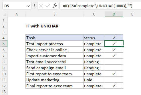
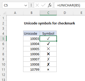
The logic of this formula is the same as the original formula above. However, instead of hardcoding a plain text version of a checkmark into the formula, the UNICHAR function is used to return the Unicode character 10003. The benefit of this approach is that you can easily change the number to display a different character. Here are a few examples of Unicode characters related to check and tick marks:
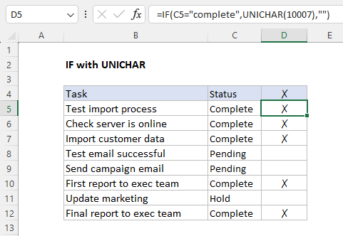
To use a different symbol, change the number in the formula. For example, use 10007 for an “X”:
=IF(C5="complete",UNICHAR(10007),"")
For more useful Unicode symbols, see: How to use the UNICHAR function .
IF with CHAR
An older way to display a checkmark in a formula is to use IF with the CHAR function , then format the result with the Wingdings font:
=IF(C5="complete",CHAR(252),"")
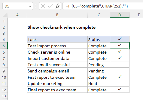
Note: with this option, you must format the range D4:D12 with the Wingdings font. If you skip this step, you will not see a checkmark. Instead, you will see a character like “ü” or similar.
With conditional formatting
You can also use Excel’s built-in conditional formatting icons to show a checkmark, but you don’t have much flexibility. Visit this page for a comprehensive guide on conditional formatting with formulas, featuring many practical examples.
Explanation
The goal is to identify dates in column B that fall between a given start date and end date. The start and end dates are exposed as inputs on the worksheet that can be changed at any time, labeled “Start” and “End” in the example shown.
Named ranges
For convenience, both start (E5) and end (E8) are named ranges that can be used directly in the formula. If you prefer not to use named ranges, use absolute references like $E$5 and $E$8 to prevent these references from changing as the formula is copied down the table.
=IF(AND(B5>=$E$5,B5<=$E$8),"x","")
Excel dates
Excel dates are just large serial numbers and can be used in any numeric calculation or comparison. This means we can compare one date to another date with a logical operator like greater than or equal (>=) or less than or equal (<=) like any other number.
AND function
The AND function returns TRUE if all arguments are TRUE. For example, if cell A1 contains “Red” and B1 contains 10, then:
=AND(A1="Red",B1>5) returns TRUE
=AND(A1="Red",B1>12) returns FALSE
=AND(A1="Blue",B1>5) returns FALSE
In this example, the main task is to construct a logical test to find dates that fall between the start and end dates. The first comparison is against the start date. We want to check if the date in B5 is greater than or equal (>=) to the date in cell E5, which is the named range start :
=B5>=start
The second expression needs to check if the date in B5 is less than or equal (<=) to the end date in cell E5:
=B5<=end
Since we want to test if both conditions are TRUE at the same time, we use the AND function like this:
=AND(B5>=start,B5<=end) // returns TRUE
For cell B5, the result is TRUE, because 11-Jan-2022 is greater than 1-Jan-2022 AND is less than 30-Apr-2022. For cell B6 however, the result is FALSE. Although 1-May-2022 is greater than 1-Jan-2022, it is not less than 30-Apr-2022:
=AND(B6>=start,B6<=end) // returns FALSE
To summarize: the AND function will return TRUE when the date in column B is greater than or equal to start (E5) AND less than equal to end (E8) If either test fails, the AND function will return FALSE. We now have the logical test we can use in the IF function.
IF function
The IF function runs a logical test and returns one value for a TRUE result, and another value for a FALSE result. The generic syntax for IF looks like this:
=IF(logical_test,if_true,if_false)
We start off by placing the expression we developed above inside the IF function as the logical_test argument:
=IF(AND(B5>=start,B5<=end),
Next, we add a value_if_true argument. In this case, we want to return an “x” when a date is between two dates, so we add “x” as a text value :
=IF(AND(B5>=start,B5<=end),"x",
If the date in B5 is not between the start and end dates, we don’t want to display anything, so we use an empty string ("") for value_if_false . The final formula in C5 is:
=IF(AND(B5>=start,B5<=end),"x","")
As the formula is copied down, the formula returns “x” if the date in column B is between the start and end date. If not, the formula returns an empty string (""), which looks like an empty cell in Excel. The values returned by the IF function can be customized as desired.
