Explanation
The goal is to return the first non-blank value in each row from columns B:E, moving left to right. One way to solve this problem is with a series of nested IF statements. Since all cells are contiguous (connected) another way to get the first value is with the XLOOKUP function. Both approaches are explained below.
Nested IF solution
In the worksheet shown, the formula in cell G5 is:
=IF(B5<>"",B5,IF(C5<>"",C5,IF(D5<>"",D5,IF(E5<>"",E5,"no value"))))
In Excel, empty double quotes ("") mean an empty string . The <> symbol is a logical operator that means “not equal to”, so the following expression means “A1 is not empty”:
=B5<>"" // B5 is not empty
The overall structure of this formula is what is called a " nested IF formula “. Each IF statement checks a cell to see if a particular cell is not empty. If a cell is not empty , the IF returns the value from that cell. If the cell is empty , the IF statement hands off processing to the following IF function. The flow of a nested IF is somewhat easier to understand if we add line breaks to the formula to separate each IF function like this:
=
IF(B5<>"",B5,
IF(C5<>"",C5,
IF(D5<>"",D5,
IF(E5<>"",E5,
"no value"))))
With ISBLANK
It is also possible to use the ISBLANK function , which returns TRUE when a cell is blank:
=ISBLANK(A1) // A1 is blank
The behavior can be “reversed” by nesting the ISBLANK function inside the NOT function :
=NOT(ISBLANK(A1)) // A1 is not blank
The original formula above can be re-written to use ISBLANK as follows:
=IF(NOT(ISBLANK(B5)),B5,IF(NOT(ISBLANK(C5)),C5,IF(NOT(ISBLANK(D5)),D5,IF(NOT(ISBLANK(E5)),E5,"no value"))))
XLOOKUP solution
Another way to solve this problem is with the XLOOKUP formula like this:
=XLOOKUP(TRUE,ISNUMBER(B5:E5),B5:E5)
We can use XLOOKUP in this case because the four cells in B5:E5 are together, so they can be provided as a single range. The ISNUMBER function checks the range and returns an array of TRUE and FALSE values like this:
{TRUE,TRUE,TRUE,TRUE}
Explanation
The goal is to “flag” records that are neither “Red” nor “Green”. More specifically, we want to check the color in column B, and leave an “x” in rows where the color is NOT “Red” OR “Green”. If the color is “Red” OR “Green”, we want to display nothing.
IF function logic
The IF function is commonly used for simple tests. For example, to return “OK”, when a value is over 100 and “Fail” if not, you can use the IF function in a formula like this:
=IF(A1>100,"OK","Fail")
In this formula, A1>100 is the logical test. The behavior of the IF function can be easily extended by adding functions like AND , OR , and NOT to the logical test. For example, to reverse the existing logic in the formula above, we can add NOT like this:
=IF(NOT(A1>100),"OK","Fail")
Translation: If the value in A1 is NOT greater than 100, then return “OK”. Otherwise, return “Fail”.
In the worksheet shown, the goal is to mark records where the color is NOT “Red” OR “Green” with an “x”. If the color is “Red” or “Green” we don’t want to do anything. The formula in cell D6 is:
=IF(NOT(OR(B6="red",B6="green")),"x","")
In this formula, the logical test is this bit:
NOT(OR(B6="red",B6="green"))
Working from the inside out, we first use the OR function to test for “red” or “green”:
OR(B6="red",B6="green")
OR will return TRUE if B6 is “Red” or “Green”, and FALSE if B6 contains any other value. The NOT function simply reverses this result. Adding NOT means the test will return TRUE if B6 is NOT “Red” or “Green”, and FALSE otherwise:
NOT(OR(B6="red",B6="green"))
The rest of the formula is standard. Since we want to flag items that pass the test, we provide “x” for value_if_true . Since we don’t want to display anything for other values, we provide an empty string (”") for value_if_false . This causes an “x” to appear in column D when the color in column B is NOT “Red” or “Green”. You can extend the OR function to check additional conditions as needed.
Keep in mind that Excel is not case-sensitive by default, so the color names in the formula are all lowercase. The expressions B6=“red”, B6=“Red”, and B6=“RED” will all return the same result. Also, notice that we need to provide an empty string ("") for the false result. This argument is not required, but if we leave it empty, the formula will return FALSE when a color is “Red” or “Green”.
Increase price
You can use other formulas inside the IF function to run a different calculation instead of simply returning “x”. For example, let’s say you want to increase the price for all colors except Red and Green by 15%. If the color is Red or Green, you want to leave the price alone. To perform this task, the formula in E6 below is:
=IF(NOT(OR(B6="red",B6="green")),C6*1.15,C6)
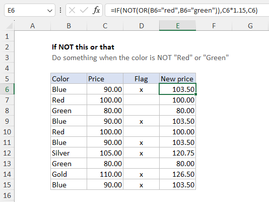
Translation: if the color is NOT “Red” or “Green”, increase the price by 15%. Otherwise, return the original price.
