Purpose
Return value
Syntax
=IFERROR(value,value_if_error)
- value - The value, reference, or formula to check for an error.
- value_if_error - The value to return if an error is found.
Using the IFERROR function
The IFERROR function returns a custom result when a formula returns an error and a normal result when a formula calculates without an error. The typical syntax for the IFERROR function looks like this:
=IFERROR(formula,custom)
In the example above, “formula” represents a formula that might return an error, and “custom” represents the value that should be returned if the formula returns an error. This makes IFERROR an elegant way to trap and manage errors in one step. Before the introduction of IFERROR, it was necessary to use more complicated nested IF statements together with the older ISERROR function .
You can use the IFERROR function to trap and handle errors produced by other formulas or functions. IFERROR checks for the following errors: #N/A, #VALUE!, #REF!, #DIV/0!, #NUM!, #NAME?, or #NULL!.
Example 1 - Trap #DIV/0! errors
In the example shown, the formula in E5 copied down is:
=IFERROR(C5/D5,0)
This formula catches the #DIV/0! error that occurs when the quantity field is empty or zero, and replaces it with zero. You are free to change the zero (0) to suit your needs. For example, to display nothing, you could use an empty string ("") instead of zero:
=IFERROR(C5/D5,"")
This version of the formula will trap the #DIV/0! error and return an empty string, which looks like an blank cell.
Example 2 - request input before calculating
Sometimes you may want to suppress a calculation until the worksheet receives specific input. For example, if A1 contains 10, B1 is blank, and C1 contains the formula =A1/B1, the following formula will return a #DIV/0 error if B1 is empty:
=IFERROR(A1/B1) // returns #DIV! if B1 is empty
The formula below has been modified to use the IFERROR function to trap the #DIV/0! error and remap it to the message “Please enter a value in B1”.
=IFERROR(A1/B1,"Please enter a value in B1")
As long as B1 is empty, C1 will display the message “Please enter a value in B1” if B1. When a number is entered in B1, the formula will return the result of A1/B1.
Example 3 - Sum and ignore errors
A common problem in Excel is that errors in data will corrupt the results of other formulas. For example, in the worksheet shown below, the goal is to sum values in the range D5:D15. However, because the range D5:D15 contains #N/A errors, the SUM function will return #N/A:
=SUM(D5:D15) // returns #N/A
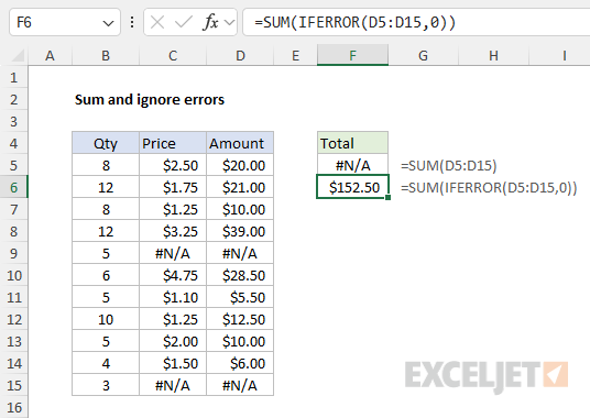
To ignore the #N/A errors and sum the remaining values, we can adjust the formula to use the IFERROR function like this:
=SUM(IFERROR(D5:D15,0)) // returns 152.50
Essentially, we use IFERROR to map the errors to zero and then sum the result. For more details and alternatives, see Sum and ignore errors .
Example 3 - VLOOKUP #N/A
When VLOOKUP cannot find a lookup value, it returns an #N/A error. You can use the IFERROR function to catch the #N/A error VLOOKUP throws when a lookup value isn’t found like this:
=IFERROR(VLOOKUP(value,data,column,0),"Not found")
In this example, the IFERROR function evaluates the result returned by VLOOKUP. If no error is present, the result is returned normally. However, if VLOOKUP returns an #N/A error, IFERROR catches the error and returns “Not Found”.
IFERROR or IFNA?
The IFERROR function is useful, but it is a rather blunt instrument that will trap all kinds of errors. For example, if a function is misspelled in a formula, Excel will return the #NAME? error and IFERROR will catch that error too, and return an alternate result. This can cause IFERROR to hide an important problem. In most cases, it makes more sense to use the IFNA function with VLOOKUP instead of IFERROR.
=IFNA(VLOOKUP(value,data,column,0),"Not found")
Unlike IFERROR, IFNA only traps the #N/A error.
Other error functions
Excel provides several error-related functions, each with a different behavior:
- The ISERR function returns TRUE for any error type except the #N/A error.
- The ISERROR function returns TRUE for any error.
- The ISNA function returns TRUE for #N/A errors only.
- The ERROR.TYPE function returns the numeric code for a given error.
- The IFERROR function traps errors and provides an alternative result.
- The IFNA function traps #N/A errors and provides an alternative result.
Notes
- If value is empty, it is evaluated as an empty string ("") and not an error.
- If value_if_error is supplied as an empty string (""), no message is displayed when an error is detected.
- In Excel 2013+, you can use the IFNA function to trap and handle #N/A errors specifically.
Purpose
Return value
Syntax
=IFNA(value,value_if_na)
- value - The value, reference, or formula to check for an error.
- value_if_na - The value to return if #N/A error is found.
Using the IFNA function
The IFNA function is designed to manage #N/A errors and ignore other errors. When a function returns an #N/A, it typically indicates that a value is not available or not found. In many cases, an #N/A error is useful information because it tells you the formula is not able to find a value. However, the #N/A error can make users uncomfortable, because it might make it seem that there something is wrong with the worksheet. The IFNA function gives you a simple way to “catch” an #N/A error and provide another more user-friendly result. Unlike the more general IFERROR function, the IFNA function will only trap #N/A errors specifically; other errors will still be displayed. This is useful because it means the IFNA function won’t accidentally hide another more serious error.
You can use the IFNA function to trap and handle #N/A errors that may occur in formulas that perform lookups, such as VLOOKUP , MATCH , HLOOKUP , etc. The IFNA function returns a custom result when a formula generates the #N/A error, and a normal result when no error is detected.
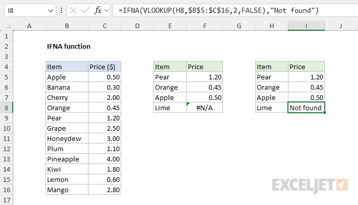
Example
For example, in the worksheet shown, we are using VLOOKUP to find an item’s price in the range B5:C16. The formula in F5, copied down, looks like this:
=VLOOKUP(E5,$B$5:$C$16,2,FALSE)
Notice the formula works fine in the first three cells, correctly returning a price for Pear, Apple, and Orange. However, in cell F8 VLOOKUP returns #N/A because there is no entry for “Lime” in column B. The #N/A result essentially means “not found”, but it is returned as an error on the worksheet. We can catch this error and return an alternative result with the IFNA function.
To use the IFNA function to trap #N/A errors, embed the original formula inside IFNA as the first argument. In this case, we start off with the IFNA function:
=IFNA(
Then we paste in the original formula like so:
=IFNA(VLOOKUP(H5,$B$5:$C$16,2,FALSE),
Next, provide an alternative result as the second argument. In the worksheet shown, we provide an empty string ("") so that the #N/A error is effectively hidden. The final formula in cell I5 looks like this:
=IFNA(VLOOKUP(H5,$B$5:$C$16,2,FALSE),"")
Notice that the result in cells I5, I6, and I7 is unaffected; VLOOKUP returns the item price as before. However, in cell I8, we now see a blank cell. Inside IFNA, VLOOKUP returns #N/A as before. IFNA detects the #N/A error and returns an empty string ("") instead, which displays like an empty cell. If you would rather display a message like “Not found”, simply modify the formula to include the message like this:
=IFNA(VLOOKUP(H5,$B$5:$C$16,2,FALSE),"Not found")
Note that the message must be enclosed in double quotes. The screen below shows how this modified formula behaves on the worksheet:
IFERROR vs IFNA
Like the IFNA function, the IFERROR function is designed to manage errors. In the worksheet shown, we can use IFERROR instead of IFNA like this:
=IFERROR(VLOOKUP(H8,$B$5:$C$16,2,FALSE),"")
Notice the structure is exactly the same. The original formula appears as the first argument inside IFERROR and the custom result ("") is the second argument. However, unlike IFNA, IFERROR will catch any error. This makes IFERROR a more blunt instrument since it will trap many kinds of errors. For example, if a function name is misspelled, Excel will normally return the #NAME? error:
=ZLOOKUP(H8,$B$5:$C$16,2,FALSE) // returns #NAME?
Above there is no function called “ZLOOKUP”, so Excel returns #NAME?. IFERROR will catch this error as well, even though it has nothing to do with the operation of the formula:
=IFERROR(ZLOOKUP(H8,$B$5:$C$16,2,FALSE),"") // returns ""
In other words, IFERROR may unintentionally hide other errors and obscure an important problem. As a result, it makes more sense to use the IFNA function if the intent is to manage #N/A errors only.
Other error functions
Excel provides a number of error-related functions, each with a different behavior:
- The ISERR function returns TRUE for any error type except the #N/A error.
- The ISERROR function returns TRUE for any error.
- The ISNA function returns TRUE for #N/A errors only.
- The ERROR.TYPE function returns the numeric code for a given error.
- The IFERROR function traps errors and provides an alternative result.
- The IFNA function traps #N/A errors and provides an alternative result.
Notes
- If value is empty, it is evaluated as an empty string ("") and not an error.
- If value_if_na is supplied as an empty string (""), no message is displayed when an error is detected.
