Purpose
Return value
Syntax
=IFNA(value,value_if_na)
- value - The value, reference, or formula to check for an error.
- value_if_na - The value to return if #N/A error is found.
Using the IFNA function
The IFNA function is designed to manage #N/A errors and ignore other errors. When a function returns an #N/A, it typically indicates that a value is not available or not found. In many cases, an #N/A error is useful information because it tells you the formula is not able to find a value. However, the #N/A error can make users uncomfortable, because it might make it seem that there something is wrong with the worksheet. The IFNA function gives you a simple way to “catch” an #N/A error and provide another more user-friendly result. Unlike the more general IFERROR function, the IFNA function will only trap #N/A errors specifically; other errors will still be displayed. This is useful because it means the IFNA function won’t accidentally hide another more serious error.
You can use the IFNA function to trap and handle #N/A errors that may occur in formulas that perform lookups, such as VLOOKUP , MATCH , HLOOKUP , etc. The IFNA function returns a custom result when a formula generates the #N/A error, and a normal result when no error is detected.
Example
For example, in the worksheet shown, we are using VLOOKUP to find an item’s price in the range B5:C16. The formula in F5, copied down, looks like this:
=VLOOKUP(E5,$B$5:$C$16,2,FALSE)
Notice the formula works fine in the first three cells, correctly returning a price for Pear, Apple, and Orange. However, in cell F8 VLOOKUP returns #N/A because there is no entry for “Lime” in column B. The #N/A result essentially means “not found”, but it is returned as an error on the worksheet. We can catch this error and return an alternative result with the IFNA function.
To use the IFNA function to trap #N/A errors, embed the original formula inside IFNA as the first argument. In this case, we start off with the IFNA function:
=IFNA(
Then we paste in the original formula like so:
=IFNA(VLOOKUP(H5,$B$5:$C$16,2,FALSE),
Next, provide an alternative result as the second argument. In the worksheet shown, we provide an empty string ("") so that the #N/A error is effectively hidden. The final formula in cell I5 looks like this:
=IFNA(VLOOKUP(H5,$B$5:$C$16,2,FALSE),"")
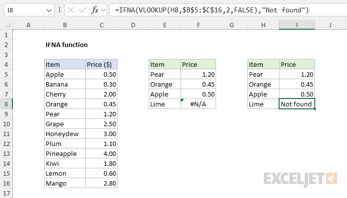
Notice that the result in cells I5, I6, and I7 is unaffected; VLOOKUP returns the item price as before. However, in cell I8, we now see a blank cell. Inside IFNA, VLOOKUP returns #N/A as before. IFNA detects the #N/A error and returns an empty string ("") instead, which displays like an empty cell. If you would rather display a message like “Not found”, simply modify the formula to include the message like this:
=IFNA(VLOOKUP(H5,$B$5:$C$16,2,FALSE),"Not found")
Note that the message must be enclosed in double quotes. The screen below shows how this modified formula behaves on the worksheet:
IFERROR vs IFNA
Like the IFNA function, the IFERROR function is designed to manage errors. In the worksheet shown, we can use IFERROR instead of IFNA like this:
=IFERROR(VLOOKUP(H8,$B$5:$C$16,2,FALSE),"")
Notice the structure is exactly the same. The original formula appears as the first argument inside IFERROR and the custom result ("") is the second argument. However, unlike IFNA, IFERROR will catch any error. This makes IFERROR a more blunt instrument since it will trap many kinds of errors. For example, if a function name is misspelled, Excel will normally return the #NAME? error:
=ZLOOKUP(H8,$B$5:$C$16,2,FALSE) // returns #NAME?
Above there is no function called “ZLOOKUP”, so Excel returns #NAME?. IFERROR will catch this error as well, even though it has nothing to do with the operation of the formula:
=IFERROR(ZLOOKUP(H8,$B$5:$C$16,2,FALSE),"") // returns ""
In other words, IFERROR may unintentionally hide other errors and obscure an important problem. As a result, it makes more sense to use the IFNA function if the intent is to manage #N/A errors only.
Other error functions
Excel provides a number of error-related functions, each with a different behavior:
- The ISERR function returns TRUE for any error type except the #N/A error.
- The ISERROR function returns TRUE for any error.
- The ISNA function returns TRUE for #N/A errors only.
- The ERROR.TYPE function returns the numeric code for a given error.
- The IFERROR function traps errors and provides an alternative result.
- The IFNA function traps #N/A errors and provides an alternative result.
Notes
- If value is empty, it is evaluated as an empty string ("") and not an error.
- If value_if_na is supplied as an empty string (""), no message is displayed when an error is detected.
Purpose
Return value
Syntax
=IFS(test1,value1,[test2, value2],...)
- test1 - First logical test.
- value1 - Result when test1 is TRUE.
- test2, value2 - [optional] Second test/value pair.
Using the IFS function
The IFs function evaluates multiple expressions and returns a result that corresponds to the first TRUE result. You can use the IFS function when you want a self-contained formula to test multiple conditions at the same time without nesting multiple IF statements. Formulas based on IFS are shorter and easier to read and write.
Conditions are provided to the IFS function as test/value pairs, and IFS can handle up to 127 conditions. Each test represents a logical test that returns TRUE or FALSE, and the value that follows will be returned when the test returns TRUE. In the event that more than one condition returns TRUE, the value corresponding to the first TRUE result is returned. For this reason, it is important to consider the order in which conditions appear.
Structure
An IFS formula with 3 tests can be visualized like this:
=IFS(
test1,value1 // pair 1
test2,value2 // pair 2
test3,value3 // pair 3
)
A value is returned by IFS only when the previous test returns TRUE, and the first test to return TRUE “wins”. For better readability, you can add line breaks to an IFS formula as shown above.
Note: the IFS function does not provide an argument for a default value. See Example #3 below for a workaround.
Example #1 - grades, lowest to highest
In the example shown below, the IFS function is used to assign a grade based on a score. The formula in E5, copied down, is:
=IFS(C5<60,"F",C5<70,"D",C5<80,"C",C5<90,"B",C5>=90,"A")
Notice the conditions are entered “in order” to test lower scores first. The grade associated with the first test to return TRUE is returned.
Example #2 - rating, highest to lowest
In a simple rating system, a score of 3 or greater is “Good”, a score between 2 and 3 is “Average”, and anything below 2 is “Poor”. To assign these values with IFS, three conditions are used:
=IFS(A1>=3,"Good",A1>=2,"Average",A1<2,"Poor")
Notice in this case, conditions are arranged to test higher values first.
Example #3 - default value
The IFS function does not have a built-in default value to use when all conditions are FALSE. However, to provide a default value, you can enter TRUE as a final test, followed by a value to use as a default.
In the example below, a status code of 100 is “OK”, a code of 200 is “Warning”, and a code of 300 is “Error”. Any other code value is invalid, so TRUE is provided as the final test, and “Invalid” is provided as a “default” value.
=IFS(A1=100,"OK",A1=200,"Warning",A1=300,"Error",TRUE,"Invalid")
When the value in A1 is 100, 200, or 300, IFS will return the messages shown above. When A1 contains any other value (including when A1 is empty) IFS will return “Invalid”. Without this final condition, IFS will return #N/A when a code is not recognized.
IFS and performance
You might expect the IFS function to “short-circuit” and stop evaluating once it finds a logical test that returns TRUE, but this is not the case. IFS evaluates all conditions and expressions , even when the first logical test is TRUE. This behavior can degrade performance when an IFS formula includes complex or time-consuming calculations, since those calculations may still run even when their conditions are FALSE. It can also cause problems in recursive LAMBDA functions, because the “else” branch is evaluated even when it should be bypassed, potentially triggering unintended recursion and a #NUM! error.
To avoid these issues, consider rewriting the formula with nested IF functions or using the simpler CHOOSE function . Both IF and CHOOSE perform true short-circuit evaluation, skipping unnecessary calculations once a valid result is found.
IFS versus SWITCH
Like the SWITCH function , the IFS function allows you to test more than one condition in a single self-contained formula. Both functions make it easier to write (and read) a formula with many conditions. One advantage of SWITCH over IFS is that the expression appears just once in the function and does not need to be repeated. In addition, SWITCH can accept a default value. However, SWITCH is limited to exact matching. It is not possible to use operators like greater than (>) or less than (<) with the standard syntax. In contrast, the IFS function requires expressions for each condition, so you can use logical operators as needed.
Notes
- The IFS function does not have a built-in default value to use when all conditions are FALSE.
- To provide a default value, enter TRUE as a final test, and a value to return when no other conditions are met.
- All logical tests must return TRUE or FALSE. Any other result will cause IFS to return a #VALUE! error.
- If no logical tests return TRUE, IFS will return the #N/A error.
- IFS does not have short-circuit behavior; all expressions are evaluated
