Income statements are commonly shown in a combo chart, with columns plotting revenue and net income, and a line showing the profit margin as a percentage. You can see examples of this on Google’s finance pages . This kind of chart is easy to make in later versions of Excel by inserting a combo chart.
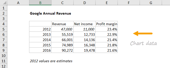
The data used to create this chart is shown below:
How to make this chart
- Select the data and insert a “combo chart”
- Select the send option - columns with line on secondary axis:
- The initial chart looks like this:
- Select revenue columns, then set series overlap and gap with
- Select legend and move to top:
- Select secondary axis and set units to major units to .01 (1%):
- Chart at this point:
At this point you can finalize the chart by setting the chart title, chart size, and font size for all text.
Bar and column charts are great for comparing things, because it’s easy to see how bar lengths differ. This chart is an example of a clustered column chart showing product units sold this year versus last year. The data used for this chart looks like this on the worksheet:

Note: you can see the same data in a clustered bar chart .
How to make this chart
- Select the data and insert a bar char on the ribbon:
- Insert the first 2D bar chart option:
- Right-click each data series and use fill tool to change color:
- After changing colors:
- Select chart data: Chart tools > Design > Select data
- Move this year series up:
- Move legend to top:
- Select data series and set overlap to zero and bar width to 60%:
- Final chart:
