Purpose
Return value
Syntax
=INDEX(array,row_num,[col_num],[area_num])
- array - A range of cells, or an array constant.
- row_num - The row position in the reference or array.
- col_num - [optional] The column position in the reference or array.
- area_num - [optional] The range in reference that should be used.
Using the INDEX function
The INDEX function returns the value at a given location in a range or array. INDEX is a powerful and versatile function. You can use INDEX to retrieve individual values or entire rows and columns. INDEX is frequently used together with the MATCH function . In this scenario, the MATCH function locates a value and feeds the numeric position to the INDEX function, and INDEX returns the value at that position.
In the most common usage, INDEX takes three arguments: array , row_num , and col_num . Array is the range or array from which to retrieve values. Row_num is the row number from which to retrieve a value, and col_num is the column number at which to retrieve a value. Col_num is optional and not needed when array is one-dimensional.
In the example shown above, the goal is to get the diameter of the planet Jupiter. Because Jupiter is the fifth planet in the list, and Diameter is the third column, the formula in G7 is:
=INDEX(B5:E13,5,3) // diameter of Jupiter
The formula above is of limited value because the row and column numbers have been hard-coded. Typically, the MATCH function would be used inside INDEX to provide these numbers. For a detailed explanation with many examples, see How to use INDEX and MATCH .
Basic usage
INDEX gets a value at a given location in a range of cells based on numeric position. When the range is one-dimensional, you only need to supply a row number. When the range is two-dimensional, you must supply both the row and column numbers. For example, to get the third item from the one-dimensional range A1:A5:
=INDEX(A1:A5,3) // returns value in A3
The formulas below show how INDEX can be used to get a value from a two-dimensional range:
=INDEX(A1:B5,2,2) // returns value in B2
=INDEX(A1:B5,3,1) // returns value in A3
INDEX and MATCH
In the examples above, the position is “hardcoded”. Typically, the MATCH function is used to find positions for INDEX. For example, in the screen below, the MATCH function is used to locate “Mars” (G6) in row 3 and feed that position to INDEX. The formula in G7 is:
=INDEX(B5:E13,MATCH(G6,B5:B13,0),3)

MATCH provides the row number (4) to INDEX. The column number is still hardcoded as 3.
INDEX and MATCH with horizontal table
In the screen below, the table above has been transposed horizontally. The MATCH function returns the column number (4) and the row number is hardcoded as 2. The formula in C10 is:
=INDEX(C4:K6,2,MATCH(C9,C4:K4,0))

For a detailed explanation with many examples, see: How to use INDEX and MATCH
Entire row / column
INDEX can be used to return entire columns or rows like this:
=INDEX(range,0,n) // entire column
=INDEX(range,n,0) // entire row
where n represents the number of the column or row to return. This example shows a practical application of this idea.
Reference as result
It’s important to note that the INDEX function returns a reference as a result. For example, in the following formula, INDEX returns A2:
=INDEX(A1:A5,2) // returns A2
In a typical formula, you’ll see the value in cell A2 as a result, so it’s not obvious that INDEX is returning a reference. However, this is a useful feature in formulas like this one , which uses INDEX to create a dynamic named range . You can use the CELL function to report the reference returned by INDEX.
Two forms
The INDEX function has two forms: array and reference . Both forms have the same behavior – INDEX returns a reference in an array based on a given row and column location. The difference is that the reference form of INDEX allows more than one array , along with an optional argument to select which array should be used. Most formulas use the array form of INDEX, but both forms are discussed below.
Array form
In the array form of INDEX, the first parameter is an array , which is supplied as a range of cells or an array constant. The syntax for the array form of INDEX is:
INDEX(array,row_num,[col_num])
- If both row_num and col_num are supplied, INDEX returns the value in the cell at the intersection of row_num and col_num .
- If row_num is set to zero, INDEX returns an array of values for an entire column. To use these array values, you can enter the INDEX function as an array formula in a horizontal range, or feed the array into another function.
- If col_num is set to zero, INDEX returns an array of values for an entire row. To use these array values, you can enter the INDEX function as an array formula in a vertical range, or feed the array into another function.
Reference form
In the reference form of INDEX, the first parameter is a reference to one or more ranges, and a fourth optional argument, area_num , is provided to select the appropriate range. The syntax for the reference form of INDEX is:
INDEX(reference,row_num,[col_num],[area_num])
Just like the array form of INDEX, the reference form of INDEX returns the reference of the cell at the intersection row_num and col_num . The difference is that the reference argument contains more than one range, and area_num selects which range should be used. The area_num is argument is supplied as a number that acts like a numeric index. The first array inside reference is 1, the second array is 2, and so on.
For example, in the formula below, area_num is supplied as 2, which refers to the range A7:C10:
=INDEX((A1:C5,A7:C10),1,3,2)
In the above formula, INDEX will return the value at row 1 and column 3 of A7:C10.
- Multiple ranges in reference are separated by commas and enclosed in parentheses.
- All ranges must on one sheet or INDEX will return a #VALUE error. Use the CHOOSE function as a workaround .
Purpose
Return value
Syntax
=INDIRECT(ref_text,[a1])
- ref_text - A reference supplied as text.
- a1 - [optional] A boolean to indicate A1 or R1C1-style reference. Default is TRUE = A1 style.
Using the INDIRECT function
The INDIRECT function converts a text string like “Sheet1!A1” into a valid reference like =Sheet1!A1 . That sounds simple enough, but of all Excel’s many functions , INDIRECT might be the most confusing to users. Why would you use text when you can simply provide a normal reference? Well, one reason is that you already have a reference as text (perhaps in a cell), and you want to make Excel understand the text as a reference . Another reason is that you want to build a dynamic reference using different bits of information. With text, it’s easy to hardcode some values, pick up other values on the worksheet, and join the values together using concatenation . The problem, however, is that once you have created a reference as text, Excel won’t recognize it as a reference. To Excel, it’s just an ordinary text value. The INDIRECT function is like a magic wand that converts a text value to an actual reference.
INDIRECT is a volatile function and can cause performance issues in large or complex worksheets.
Quick syntax demo
INDIRECT takes two arguments , in a generic syntax like this:
=INDIRECT(ref_text,[a1])
Ref_text is the text string to evaluate as a reference. The second argument, a1 , is optional and indicates the “style” of the reference provided. When a1 is omitted (or TRUE), INDIRECT evaluates ref_text as an “A1” style reference. When a1 is FALSE, INDIRECT evaluates ref_text as an “R1C1” style reference. For example:
=INDIRECT("A1") // returns a reference to A1
=INDIRECT("C5") // returns a reference to C5
=INDIRECT("R1C1",FALSE) // returns a reference to A1
=INDIRECT("R5C3",FALSE) // returns a reference to C5
Note: the a1 argument only changes the way INDIRECT evaluates ref_text, not the result.
Things to know about INDIRECT
Here are some things you should know about the INDIRECT function:
- The input to INDIRECT is text . You can create this text any way you like.
- INDIRECT will evaluate the text and convert it into a valid reference .
- If INDIRECT can’t understand the text as a reference, it will return a #REF error.
- INDIRECT can cause performance problems in large or complex worksheets. Use with care.
Here are a few ways you can use the INDIRECT function in a formula:
- Create a formula that uses a sheet name entered in a cell.
- Create a lookup formula with a variable lookup table.
- A formula that can assemble a cell reference from bits of text
- Create a fixed reference that will not change even when rows or columns are deleted
- Create numeric arrays with the ROW function in older versions of Excel.
Example 1 - the basic idea of INDIRECT
The worksheet below shows the basic idea of the INDIRECT function. The text entered in column E represents different ranges. However, if we try to use the text directly in the SUM function as a range, SUM returns zero:
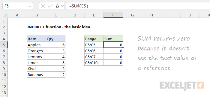
This happens because SUM doesn’t see the text value as a reference; it simply sees a text string:
=SUM(E6)
=SUM("C5:C6")
=0
The solution is to add the INDIRECT function, which converts the text values into actual ranges:
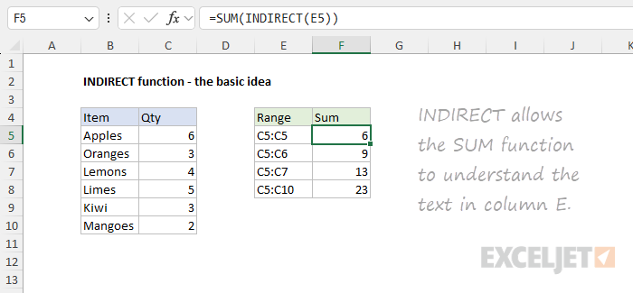
Notice in the second line below, we still have a text value, but in the third line we have the range C5:C6, and SUM now returns 9:
=SUM(INDIRECT(E6))
=SUM(INDIRECT("C5:C6"))
=SUM(C5:C6)
=9
Example 2 - Variable worksheet name
In the example shown below, INDIRECT is set up to use a variable sheet name. The formula in cell C5 is:
=INDIRECT(B5&"!A1") // sheet name in B5 is variable
The formula in C5 concatenates the text in B5 to the string “!A1” and returns the result to INDIRECT. The INDIRECT function then evaluates the text and converts it to a valid reference. As the formula is copied down, it returns the value in cell A1 for each of the 5 sheets listed in column B.
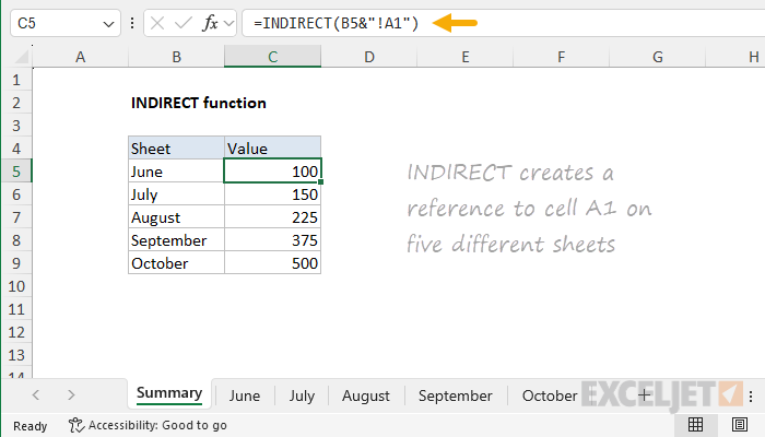
The formula is dynamic and responds to the sheet names in column B. If the sheet names are changed, the formula will automatically recalculate.
Note: As explained in this example , sheet names that contain punctuation or spaces must be enclosed in single quotes (’). This is not specific to the INDIRECT function; the same limitation is true in all formulas. The modified formula is below.
If the sheet names in your worksheet include spaces or punctuation, use the formula below:
=INDIRECT("'"&B5&"'!A1") // single quotes added
Example 3 - INDIRECT with a dropdown list
Using the same approach explained in the example above, we can allow a user to select a sheet name from a dropdown list and then construct a reference to cell A1 on the selected sheet with INDIRECT. The formula in cell C5 is the same:
=INDIRECT(B5&"!A1") // sheet name from dropdown

When a different sheet name is selected, the formula will recalculate. First, the sheet name in cell B5 will be concatenated to the text “!A1” to produce a text string like “August!A1”. Next, INDIRECT will convert the text into a regular reference like =August!A1 . Note that cell A1 is used only as an example. You can change the cell reference as desired.
Example 4 - Variable lookup table
In the worksheet below, VLOOKUP is used to get costs for two vendors, A and B. Using the vendor indicated in column F, VLOOKUP automatically uses the correct table:
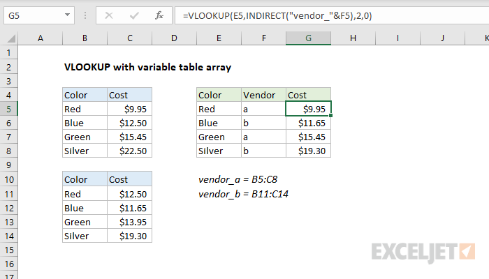
The formula in G5 is:
=VLOOKUP(E5,INDIRECT("vendor_"&F5),2,0)
Read a full explanation here .
Example 5 - Fixed reference
Normally, a reference like A1:A100 will change if rows or columns are deleted. For example, if a row is deleted in this range, the reference will become A1:A99. To create a reference that will not change, you can use the INDIRECT function like this:
=INDIRECT("A1:A100") // fixed reference
Because the text value is static, the reference created by INDIRECT will not change even when cells, rows, or columns are inserted or deleted. The formula below will always refer to the first 100 rows of column A.
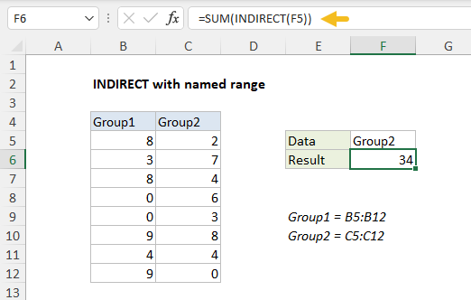
Example 6 - named range
The INDIRECT function can easily be used with named ranges. The worksheet below contains two named ranges : Group1 (B5:B12) and Group2 (C5:C12). When “Group1” or “Group2” is entered in cell F5, the formula in cell F6 sums the appropriate range using INDIRECT like this:
=SUM(INDIRECT(F5))
The value in F5 is text, but INDIRECT converts the text into a valid range.
A specific example of this approach is using named ranges to make dependent dropdown lists .
Example 7 - Generate a numeric array
A more advanced use of INDIRECT is to create a numeric array with the ROW function, like this:
ROW(INDIRECT("1:10")) // create {1;2;3;4;5;6;7;8;9;10}
One use case is explained in this formula , which sums the bottom n values in a range. You may also run into the ROW + INDIRECT approach in more complex formulas that need to assemble a numeric array “on the fly”. One example is this formula, designed to strip numeric characters from a string .
Note: this approach only makes sense in older versions of Excel. In the current version of Excel, you can easily create a numeric sequence with the SEQUENCE function .
Troubleshooting INDIRECT
Working with the INDIRECT function can be tricky because you can’t actually see the reference it returns. Instead, you just see the value at the reference when it works, or an error if the reference is invalid. Here are some troubleshooting tips:
- Be sure you have a good understanding of How to concatenate in Excel . Many INDIRECT problems are caused by text values that can’t be coerced into a valid reference.
- Be sure to include single quotes when referencing sheet names that contain spaces or punctuation (i.e., ‘Sheet 1’!A1 ).
- Debug the text string being delivered to INDIRECT with the F9 key to confirm it meets expectations.
- Work in small steps to make sure INDIRECT is returning the reference you expect before plugging it into a more complex formula.
Notes
- References created by INDIRECT are evaluated in real-time, and the value at the reference is returned.
- When ref_text is an external reference to another workbook, the workbook must be open.
- When a1 is TRUE (the default value), INDIRECT evaluates ref_text as an “A1” style reference.
- When a1 is FALSE, INDIRECT evaluates ref_text as an “R1C1” style reference.
- INDIRECT is a volatile function and can cause performance issues in large or complex worksheets.
