Explanation
Excel does not provide a formula function to append or combine ranges, either horizontally or vertically. You can use Power Query for this task, and this makes sense for data transformations that must be automated and repeated on an on-going basis. However, you can also use the LAMBDA function to create a custom function to combine ranges. This makes sense when you have good control over the data and need a solution that updates automatically, without a refresh step.
In the example below, the formula in cell C5 is:
=AppendRangeHorizontal(B5:C12,E5:F10,"")
This is a custom function created with LAMBDA, based on several Excel functions, including INDEX , SEQUENCE , IFERROR , ROWS , COLUMNS , and MAX . Holding the whole thing together are LAMBDA and LET :
=LAMBDA(range1,range2,default,
  LET(
  rows1,ROWS(range1),
  rows2,ROWS(range2),
  cols1,COLUMNS(range1),
  cols2,COLUMNS(range2),
  rowindex,SEQUENCE(MAX(rows1,rows2)),
  colindex,SEQUENCE(1,cols1+cols2),
  result,
  IF(
    colindex<=cols1,
    INDEX(range1,rowindex,colindex),
    INDEX(range2,rowindex,colindex-cols1)
  ),
  IFERROR(result,default)
  )
)
This formula is based on a formula explained here , adapted to work with columns instead or rows. It’s a good example of how the LAMBDA function and LET function work well together. Inside the LET function, the first six lines of code simply assign values to variables. Once values are assigned, these variables drive the output of the function.
The core logic of the formula, the code that builds the combined array, is here:
result,
  IF(
    colindex<=cols1,
    INDEX(range1,rowindex,colindex),
    INDEX(range2,rowindex,colindex-cols1)
  ),
  IFERROR(result,default)
  )
This code can be tricky to read, especially if you’re new to LAMBDA functions and dynamic array formulas in general. With line breaks added for readability, it’s tempting to read it like a loop, with colindex as an incrementing counter, but colindex is not one value, but an array of 4 values, created with the SEQUENCE function earlier:
colindex,SEQUENCE(1,cols1+cols2) // returns {1,2,3,4)
Similarly, rowindex is an array of 8 numbers:
rowindex,SEQUENCE(rows1+rows2) // returns {1;2;3;4;5;6;7;8}
The IF function tests the values in colindex all at once. If colindex is less than or equal to the count of the columns in range1 (2), INDEX fetches columns from range1 . If the colindex is greater than 2, INDEX fetches columns from range2 . In both cases, rowindex is used to retrieve rows.
The array that IF and INDEX create is assigned to the variable result , which is returned as a final value by the formula through the IFERROR function . This is done as a way to catch errors that occur when ranges of different row or column counts are combined. In this case, INDEX will throw an error when it tries to get a value from a non-existent row or column, and the default value will be output instead of the error.
Explanation
Excel does not provide a dedicated “contains” function, but you can create a custom function to test if a cell contains one or many strings with the LAMBDA function . LAMBDA functions do not require VBA, but are only available in Excel 365 .
The first step in creating a custom LAMBDA function is to verify the logic needed with a Excel standard formula. This LAMBDA formula is based on a Excel formula created with three functions: SUMPRODUCT , ISNUMBER , and SEARCH :
=SUMPRODUCT(--ISNUMBER(SEARCH(things,A1)))>0
Read a detailed description here . Because the LAMBDA function is only available in the dynamic array version of Excel , which handles array formulas natively, we are using SUM instead of SUMPRODUCT ( see note below ), and renaming “things” to “strings” to make the formula arguments a bit more natural:
=SUM(--ISNUMBER(SEARCH(strings,A1)))>0 // base formula
The screen below shows this formula in use with three strings “red”, “blue”, and “green”:
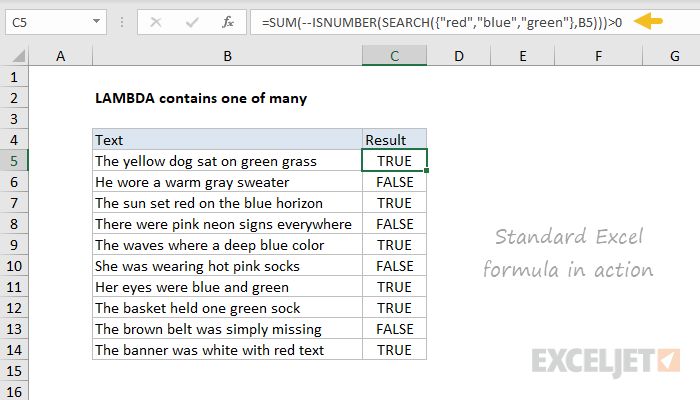
This formula returns TRUE for any cell in column B that contains any one of the strings “red”, “blue”, or “green”.
The next step is to convert this formula into a generic (unnamed) LAMBDA formula. We will need two input parameters, one for the text, and one for the strings to test. These need to appear as the first arguments in the LAMBDA formula. The final argument contains the calculation to perform, which is adapted from our standard Excel formula above. Here is the generic LAMBDA:
=LAMBDA(text,strings,SUM(--ISNUMBER(SEARCH(strings,text)))>0)
The screen below shows this formula in action, with the testing syntax needed to provide values for text and strings:
=LAMBDA(text,strings,SUM(--ISNUMBER(SEARCH(strings,text)))>0)(B5,{"red","blue","green"})
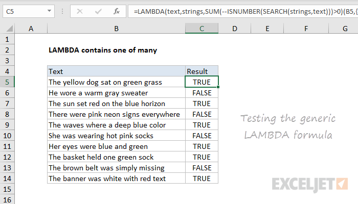
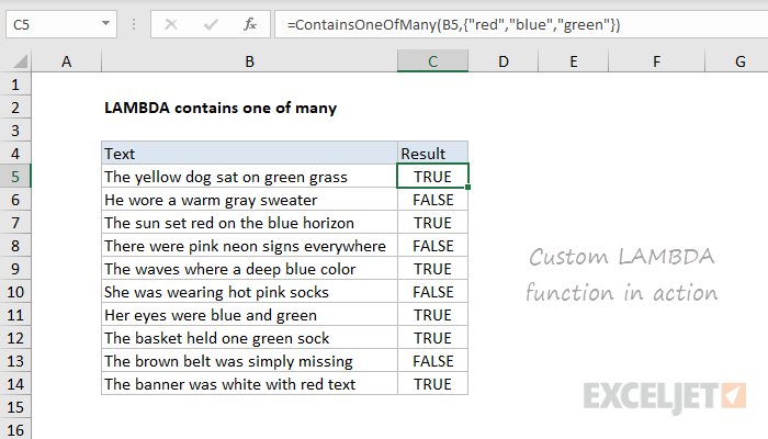
Note that results are the same as above. The next step in creating a custom LAMBDA is to name and define the formula with the Name Manager . In this case, we’ll use the name “ContainsOneOfMany”:

Finally, we update the worksheet to use the new custom function, and confirm that results are the same:
Notes
=ContainsOneOfMany(A1,range)
In addition, the formula will also work correctly if we supply only one string:
=ContainsOneOfMany(A1,"red")
Note: Traditionally, SUMPRODUCT is often seen in array formulas, because it can handle arrays natively, without control + shift + enter. This makes the formula “more friendly” to most users. The SUM function can also be used in these cases, but the formula must then be entered with control + shift + enter. In Excel 365, the SUM function will work in these cases without any special handling. Since LAMBDA is only available in Excel 365 , this example uses SUM, since SUMPRODUCT provides no additional benefit.
