Explanation
Excel does not provide a dedicated “contains” function, but you can create a custom function to test if a cell contains one or many strings with the LAMBDA function . LAMBDA functions do not require VBA, but are only available in Excel 365 .
The first step in creating a custom LAMBDA function is to verify the logic needed with a Excel standard formula. This LAMBDA formula is based on a Excel formula created with three functions: SUMPRODUCT , ISNUMBER , and SEARCH :
=SUMPRODUCT(--ISNUMBER(SEARCH(things,A1)))>0
Read a detailed description here . Because the LAMBDA function is only available in the dynamic array version of Excel , which handles array formulas natively, we are using SUM instead of SUMPRODUCT ( see note below ), and renaming “things” to “strings” to make the formula arguments a bit more natural:
=SUM(--ISNUMBER(SEARCH(strings,A1)))>0 // base formula
The screen below shows this formula in use with three strings “red”, “blue”, and “green”:
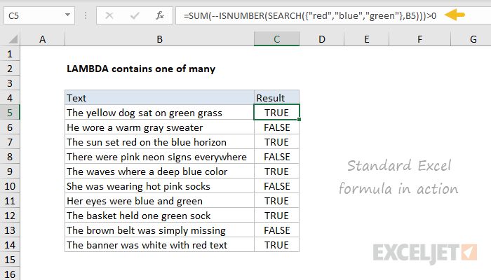
This formula returns TRUE for any cell in column B that contains any one of the strings “red”, “blue”, or “green”.
The next step is to convert this formula into a generic (unnamed) LAMBDA formula. We will need two input parameters, one for the text, and one for the strings to test. These need to appear as the first arguments in the LAMBDA formula. The final argument contains the calculation to perform, which is adapted from our standard Excel formula above. Here is the generic LAMBDA:
=LAMBDA(text,strings,SUM(--ISNUMBER(SEARCH(strings,text)))>0)
The screen below shows this formula in action, with the testing syntax needed to provide values for text and strings:
=LAMBDA(text,strings,SUM(--ISNUMBER(SEARCH(strings,text)))>0)(B5,{"red","blue","green"})
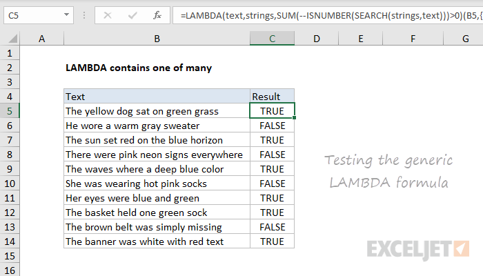
Note that results are the same as above. The next step in creating a custom LAMBDA is to name and define the formula with the Name Manager . In this case, we’ll use the name “ContainsOneOfMany”:

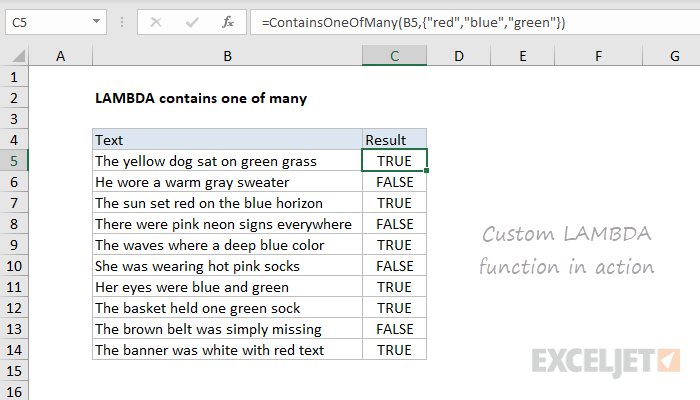
Finally, we update the worksheet to use the new custom function, and confirm that results are the same:
Notes
=ContainsOneOfMany(A1,range)
In addition, the formula will also work correctly if we supply only one string:
=ContainsOneOfMany(A1,"red")
Note: Traditionally, SUMPRODUCT is often seen in array formulas, because it can handle arrays natively, without control + shift + enter. This makes the formula “more friendly” to most users. The SUM function can also be used in these cases, but the formula must then be entered with control + shift + enter. In Excel 365, the SUM function will work in these cases without any special handling. Since LAMBDA is only available in Excel 365 , this example uses SUM, since SUMPRODUCT provides no additional benefit.
Explanation
The goal in this example is to use a formula to report which things exist in a cell. The list of things to check for is in the named range things (E5:E9). The result is returned as a comma separated text string.
The first step in creating a custom function with the LAMBDA function is to verify the logic needed to solve the problem. The formula below will do the job and return the result seen in column C:
=TEXTJOIN(", ",1,FILTER(things,ISNUMBER(SEARCH(things,B5)),""))
This formula uses four separate functions: TEXTJOIN , FILTER , ISNUMBER , and SEARCH . The core search logic is explained in detail here . FILTER catches the output from SEARCH and returns a list of matching strings, and TEXTJOIN concatenates the values together and returns a final result.
Thinking about the logic in a more general way, we can see that there are at least four potential inputs: the text to process, the things to look for, the delimiter to use when joining final result, and a default value to return if the formula finds no matches. The formula below is a direct port to LAMBDA syntax, with the four inputs above as set up as named arguments:
=LAMBDA(text,things,delim,default,TEXTJOIN(delim,1,FILTER(things,ISNUMBER(SEARCH(things,text)),default)))
Notice the four inputs above have been defined as function arguments. Once this generic version of the function is named and defined with the Name Manager , the custom function can be used like this:
=ContainsWhichThings(B5,things,", ","")
with the same result as before.
Adding a sort option
In the LAMBDA example above, the primary benefit of making a custom function is ease of use: the custom function is easier to call and configure than the original formula.
However, if we extend the formula to sort results in the order things were found in the text, the base formula becomes significantly more complex and redundant:
=TEXTJOIN(", ",1,SORTBY(FILTER(things,ISNUMBER(SEARCH(things,B5)),""),SEARCH(FILTER(things,ISNUMBER(SEARCH(things,B5)),""),B5)))
In this version, we sort the list returned by FILTER by the position at which things occur in the text. We do this with the SORTBY function and the main complication is in creating a sort_by argument, which is done here:
SEARCH(FILTER(things,ISNUMBER(SEARCH(things,B5)),""),B5) // sort_by
Notice the code inside the outer SEARCH repeats code already in the formula. To clean things up, we’ll want to use the LET function , but first, we’ll update the existing LAMBDA code to use the new sort logic:
=LAMBDA(text,things,delim,default,
  TEXTJOIN(", ",1,
    SORTBY(
      FILTER(things,ISNUMBER(SEARCH(things,text)),""),
      SEARCH(FILTER(things,ISNUMBER(SEARCH(things,text)),""),text))
  )
)(B5,things,", ","")
The generic function above works fine, but is still redundant. We can reduce the redundant code by assigning intermediate results to variables with the LET function. Below is a refactored version of the formula above:
=LAMBDA(text,things,delim,default,
LET(
  searchResults,FILTER(things,ISNUMBER(SEARCH(things,text)),""),
  sortedResults,SORTBY(searchResults,SEARCH(searchResults,text)),
  result,TEXTJOIN(", ",1,sortedResults),
  result
  )
)(B5,things,", ","")
Notice the primary FILTER(ISNUMBER(SEARCH())) code only appears once now, and the result is assigned to the variable “searchResults”, which is used twice in the line below. Next, we’ll make the sort optional, by adding a new argument called sort :
=LAMBDA(text,things,delim,default,sort,
LET(
  searchResults,FILTER(things,ISNUMBER(SEARCH(things,text)),""),
  sortedResults,IF(sort,
  SORTBY(searchResults,SEARCH(searchResults,text)),searchResults),
  result,TEXTJOIN(", ",1,sortedResults),
  result
  )
)(B5,things,", ","",TRUE)
The sort argument acts like a toggle. When sort is TRUE, the function will sort search results in the order they appear in text. When sort is FALSE, the function will leave the list unsorted, and found items will appear in their original order (i.e. the order they are listed in “things”). The logic for this is handled by the IF function . This is a good example of how the LAMBDA and LET functions together make it possible to extend the behavior of a custom function.
The screen below shows the new version of the formula in action. Notice the sort argument has been set to TRUE, so results are now sorted in the order they appear in text:

