Purpose
Return value
Syntax
=LAMBDA(parameter,...,calculation)
- parameter - An input value for the function.
- calculation - The calculation to perform as the result of the function. Must be the last argument.
Using the LAMBDA function
The LAMBDA function provides a way to create a custom function in Excel. Once defined and named, a LAMBDA function can be used anywhere in a workbook. LAMBDA functions can be very simple or quite complex, stringing together many Excel functions into one formula. A custom LAMBDA function does not require VBA or macros.
LAMBDA is a new function available in Excel 365 only.
Example 1 | Example 2 | Example 3 | Example 4
In computer programming, the term “lambda” refers to an anonymous function or expression. An anonymous function is a function defined without a name. In Excel, the LAMBDA function is first used to create a generic (unnamed) formula. Once a generic version has been created and tested, it is ported to the Name Manager, where it is formally defined and named.
One of the key benefits of a custom LAMBDA function is that the logic contained in the formula exists in just one place. This means there is just one copy of code to update when fixing problems or updating functionality, and changes will automatically propagate to all instances of the LAMBDA function in a workbook.
The LET function is often used together with the LAMBDA function. LET provides a way to declare variables and assign values in a formula. This makes more complicated formulas easier to read by reducing redundant code. The LET function can also improve performance by reducing the number of calculations performed by a formula.
By default, all arguments in a LAMBDA function are required. To create optional arguments, see the ISOMITTED function .
Creating a LAMBDA function
LAMBDA functions are typically created and debugged in the formula bar on a worksheet, then moved into the name manager to assign a name that can be used anywhere in a workbook.
There are four basic steps to creating and using a custom LAMBDA function:
- Verify the logic you will use with a standard formula
- Create and test a generic (unnamed) LAMBDA version of the formula
- Name and define the LAMBDA formula with the name manager
- Call the new custom function with the defined name
The examples below discuss these steps in more detail.
Example 1 - basic example
To illustrate how LAMBDA works, let’s begin with a very simple formula:
=x*y // multiply x and y
In Excel, this formula would typically use cell references like this:
=B5*C5 // with cell references

As you can see, the formula works fine, so we are ready to move on to creating a generic LAMBDA formula (unnamed version). The first thing to consider is if the formula requires inputs (parameters). In this case, the answer is “yes” – the formula requires a value for x, and a value for y. With that established, we start off with the LAMBDA function, then add the required parameters for user input:
=LAMBDA(x,y // begin with input parameters
Next, we need to add the actual calculation, x*y:
=LAMBDA(x,y,x*y)
If you enter the formula at this point, you’ll get a #CALC! error. This happens because the formula has no input values to work with since there are no longer any cell references. To test the formula, we need to use a special syntax like this:
=LAMBDA(x,y,x*y)(B5,C5) // testing syntax
This syntax, where parameters are supplied at the end of a LAMBDA function in a separate set of parentheses, is unique to LAMBDA functions. This allows the formula to be tested directly on the worksheet before the LAMBDA is named. In the screen below, you can see that the generic LAMBDA function in F5 returns exactly the same result as the original formula in E5:

We are now ready to name the LAMBDA function with the Name Manager . First, copy the formula, but do not include the testing parameters at the end. Next, open the Name Manager with the shortcut Control + F3 , and click New.

In the New Name dialog, enter the name “XBYY”, leave the scope set to “Workbook”, and paste the formula you copied into the “Refers to” input area. (Tip: Use the tab key to navigate to the “Refers to” field).

Make sure the formula begins with an equals sign (=). Now that the LAMBDA formula has a name, it can be used in the workbook like any other function. In the screen below, the formula in G5, copied down, is:
=XBYY(B5,C5)
The screen below shows how things look in the workbook:

The new custom function returns the same result as the other two formulas.
Custom LAMBDA names have certain restrictions you should be aware of.
Example 2 - volume of sphere
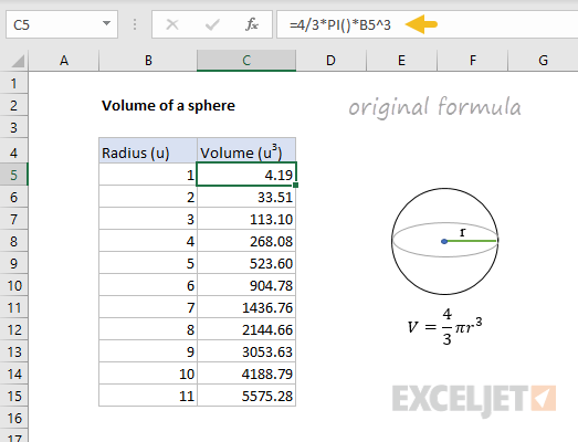
In this example, we’ll convert a formula to calculate the volume of a sphere into a custom LAMBDA function. The general Excel formula for calculating the volume of a sphere is:
=4/3*PI()*A1^3 // volume of sphere
where A1 represents the radius. The screen below shows this formula in action:
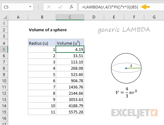
Notice this formula only requires one input (radius) to calculate volume, so our LAMBDA function will only need one parameter (r), which will appear as the first argument. Here is the formula converted to LAMBDA:
=LAMBDA(r,4/3*PI()*r^3) // generic lambda
Back in the worksheet, we’ve replaced the original formula with the generic LAMBDA version. Notice we are using the testing syntax, which allows us to plug in B5 for radius:
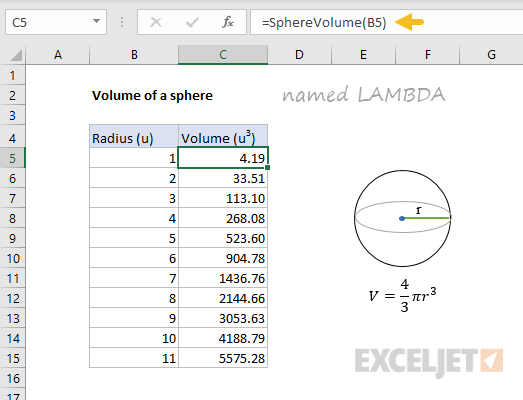
The results from the generic LAMBDA formula are exactly the same as the original formula, so the next step is to define and name this LAMBDA formula with the Name Manager , as explained above. The name used for a LAMBDA function can be any valid Excel name. In this case, we’ll name the formula “SphereVolume”.
Back in the worksheet, we’ve replaced the generic (unnamed) LAMBDA formula with the named LAMBDA version and entered B5 for r. Notice that the results returned by the custom SphereVolume function are exactly the same as those of previous results.
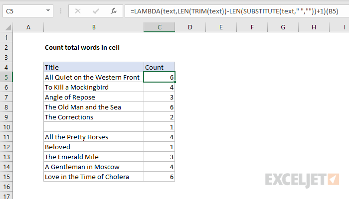
Example 3 - count words
In this example, we’ll create a LAMBDA function to count words. Excel doesn’t have a function for this purpose, but you can count words in a cell with a custom formula based on the LEN and SUBSTITUTE functions like this:
=LEN(TRIM(A1))-LEN(SUBSTITUTE(A1," ",""))+1
Read the detailed explanation here . Here is the formula in action in a worksheet:
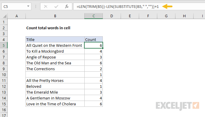
Notice we get an incorrect count of 1 when the formula is given an empty cell (B10). We’ll address this problem below.
This formula only requires one input: the text containing words. In our LAMBDA function, we’ll name this argument “text”. Here is the formula converted to LAMBDA:
=LAMBDA(text,LEN(TRIM(text))-LEN(SUBSTITUTE(text," ",""))+1)
Notice “text” appears as the first argument, and the calculation is the second and final argument. In the screen below, we’ve replaced the original formula with the generic LAMBDA version. Notice we are using the testing syntax, which allows us to plug in B5 for text:
=LAMBDA(text,LEN(TRIM(text))-LEN(SUBSTITUTE(text," ",""))+1)(B5)
The results from the generic LAMBDA formula are the same as the original formula, so the next step is to define and name this LAMBDA formula with the Name Manager , as explained previously. We’ll name this formula “CountWords”.
Below, we’ve replaced the generic (unnamed) LAMBDA formula with the named LAMBDA version, and entered B5 for text. Notice we get exactly the same results.
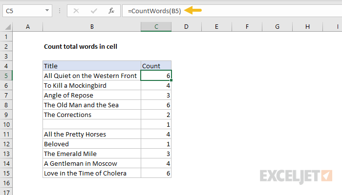
The formula used in the Name Manager to define CountWords is the same as above, without the testing syntax:
=LAMBDA(text,LEN(TRIM(text))-LEN(SUBSTITUTE(text," ",""))+1)
Fixing the empty cell problem
As mentioned above, the formula above returns an incorrect count of 1 when a cell is empty. This problem can be fixed by replacing +1 with the code below:
=LEN(TRIM(B5))-LEN(SUBSTITUTE(B5," ",""))+(LEN(TRIM(B5))>0)
Full explanation here . To update the existing named LAMBDA formula, we again need to use the Name Manager:
- Open the Name Manager
- Select the name “CountWords” and click “Edit”
- Replace the “Refers to” code with this formula:
=LAMBDA(text,LEN(TRIM(text))-LEN(SUBSTITUTE(text," ",""))+(LEN(TRIM(text))>0))
Once the Name Manager is closed, the CountWords works correctly on empty cells, as seen below:
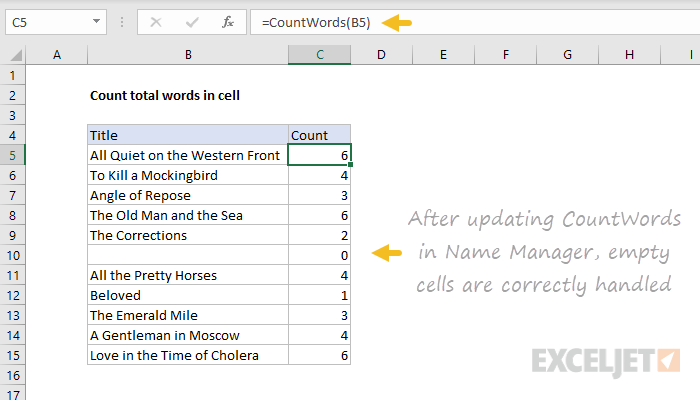
Note: Updating the code once in the Name Manager updates all instances of the CountWords formula at once. This is a key benefit of custom functions created with LAMBDA – formula updates can be managed in one place.
Example 4 - Number to words
Custom LAMBDA functions can be quite sophisticated, and they can even include sub-routines that encapsulate reusable logic. In the worksheet below, “NumberToWords” is a custom lambda that will convert a number like 123 into “One hundred twenty three” or “One hundred twenty three dollars” when currency is specified as USD:
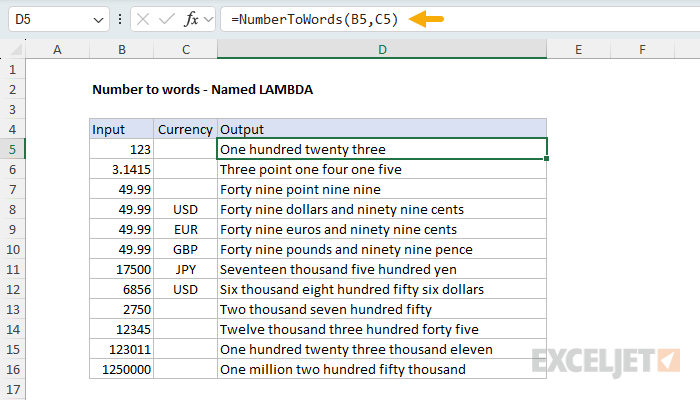
This is a complex problem in Excel, usually handled with VBA (Visual Basic). In this case, however, all required logic is contained in a single LAMBDA with about 80 lines of code. This is what the code looks like in the Excel Labs Advanced Formula Environment:

You can find the full source code and a downloadable workbook on this page .
LAMBDA naming rules
When naming a custom LAMBDA function in Excel, there are some restrictions you should be aware of:
- The name must be between 1 to 255 characters long.
- The name must start with a letter (A-Z, a-z) or an underscore (_).
- The name must not contain spaces or special characters like @, !, #, $, %, etc.
- The name must not be a cell reference like A1, C2, X100, etc.
- The name must not conflict with an existing Excel function like SUM, COUNT, TEXT, etc.
The last point, 5, is especially important. While Excel will stop you from breaking the first 4 rules, it will not prevent you from naming your custom LAMBDA after an existing function. If you break this rule, the name will be created, but your custom function will never be invoked since Excel will default to existing function names. The result can be very confusing. Avoid this trouble by making sure your custom function name is unique.
Be aware that custom LAMBDA names are case-sensitive . The names “MYFUNCTION”, “MyFunction”, and “myfunction”, are all considered unique names for a custom LAMBDA.
Purpose
Return value
Syntax
=LET(name1,value1,[name2/value2],...,result)
- name1 - First name to assign. Must begin with a letter.
- value1 - The value or calculation to assign to name 1.
- name2/value2 - [optional] Second name and value. Entered as a pair of arguments.
- result - A calculation or a variable previously calculated.
Using the LET function
The LET function lets you define named variables in a formula. There are two primary reasons you might want to do this: (1) to improve performance by eliminating redundant calculations and (2) to make more complex formulas easier to read and write. Once a variable is named, it can be assigned a static value or a value based on a calculation. The formula can then refer to a variable by name as many times as needed, while the value of the variable is defined in one place only.
Example 1 | Example 2 | Example 3 | Example 4 | More examples
Variables are named and assigned values in pairs, separated by commas (name1,value1, name2,value2, etc). LET can handle up to 126 name/value pairs, but only the first name/value pair is required. The scope of each variable is the current LET function and nested functions below. The final result is a calculation or a variable previously calculated. The result from LET always appears as the last argument to the function.
The names used in LET must begin with a letter and are not case-sensitive. You can use names that contain numbers like “count1”, “count2”, etc., but names like “ct1” and “ct2” will fail because Excel will interpret the names as a cell reference. Space characters and punctuation symbols are not allowed in names, but the underscore character (_) can be used.
The LET function is often combined with the LAMBDA function as a way to make a complex formula easier to use. LAMBDA provides a way to name a formula and reuse it in a worksheet like a custom function. Example here .
Key Benefits
The LET function provides three key benefits:
- Clarity - naming variables used in a formula can make a complex formula much easier to read and understand.
- Simplification - naming and defining variables in just one place helps eliminate redundancy and the errors that arise from having the same code in more than one place.
- Performance - elimination of redundant code means less calculation time overall since expensive calculations only need to occur once.
Example #1
Below is the general form of the LET function with one variable:
=LET(x,10,x+1) // returns 11
With a second variable:
=LET(x,10,y,5,x+y) // returns 15
After x and y have been declared and assigned values, the calculation provided in the 5th argument returns 15.
Example #2
A chief benefit of the LET function is simplification by eliminating redundancy. For example, the screenshot above shows a formula that uses the SEQUENCE function to generate all dates between May 1, 2020 and May 15, 2020, which are then filtered by the FILTER function to include only weekdays. The formula in E5 is:
=LET(dates,SEQUENCE(C5-C4+1,1,C4,1),FILTER(dates,WEEKDAY(dates,2)<6))
The first argument declares the variable dates and the second argument assigns the output from SEQUENCE to dates :
=LET(dates,SEQUENCE(C5-C4+1,1,C4,1)
Notice the start and end dates come from cells C4 and C5, respectively. Once dates has been assigned a value, it can be used in the final calculation, which is based on the FILTER function:
FILTER(dates,WEEKDAY(dates,2)<6)) // filter out weekends
Notice dates is used twice in this snippet: once by FILTER, once by the WEEKDAY function . In the first instance, the raw dates from SEQUENCE are passed into the FILTER function as the array to filter. In the second instance, the dates from SEQUENCE are passed into the WEEKDAY function, which tests for weekdays (i.e. not Sat or Sun). The result from WEEKDAY is the logic used to filter the original dates.
Without the LET function, SEQUENCE would need to appear twice in the formula, both times with the same (redundant) configuration. The LET function allows the SEQUENCE function to appear and be configured just once in the formula.
More examples
- For an example of how LET can make a tricky formula easier to follow, see this page .
- For a more complex example of how LET can eliminate redundancy, see this example .
