Explanation
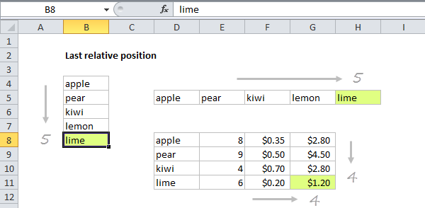
When building advanced formulas that use dynamic ranges, it’s often necessary to figure out the last location of data in a list. Depending on the data, this could be the last row with data, the last column with data, or the intersection of both. Note: we want the last relative position inside a given range , not the row number on the worksheet. The screen below shows the idea:
This formula uses the MATCH function in approximate match mode to locate the last numeric value in a range. Approximate match enabled by setting by the 3rd argument in MATCH to 1, or omitting this argument, which defaults to 1.
The lookup value is a so-called “big number” (sometimes abbreviated “bignum”) which is intentionally larger than any value that will appear in the range.
The result is that MATCH will “step back” to the last numeric value in the range, and return that position.
Note: this approach works fine with empty cells in the range, but is not reliable with mixed data that includes both numbers and text.
About bignum
The biggest number Excel can handle is 9.99999999999999E+307.
When using MATCH this way, you can use any large number that is guaranteed to be larger than any value in the range, for example:
=MATCH(1E+06,range) // 1 million
=MATCH(1E+09,range) // 1 billion
=MATCH(1E+12,range) // 1 trillion
The advantage to using 9.99E+307 or similar, is that it’s (1) a huge number and (2) recognizable as a placeholder for a “big number”. You’ll see it used in various advanced Excel formulas.
Dynamic range
You can use this formula to create a dynamic range with other functions like INDEX and OFFSET. See links below for examples and explanation:
- Dynamic range with INDEX and COUNTA
- Dynamic range with OFFSET and COUNTA
Inspiration for this article came from Mike Girvin’s excellent book Control + Shift + Enter , where Mike explains the concept of “last relative position”.
Explanation
This formula uses the MATCH function in approximate match mode to locate the last text value in a range. Approximate match enabled by setting by the 3rd argument in MATCH to 1, or omitting this argument, which defaults to 1.
The lookup value is a so-called “big text” (sometimes abbreviated “bigtext”) which is intentionally a value “bigger” than any value that will appear in the range. When working with text, which sorts alphabetically, this means a text value that will always appear at the end of the alphabetic sort order.
Since this formula matches text, the idea is to construct a lookup value that will never occur in the actual text, but will always be last. To do that, we use the REPT function to repeat the letter “z” 255 times. The number 255 represents the largest number of characters that MATCH allows in a lookup value.
When MATCH can’t find this value, it will “step back” to the last text value in the range, and return the position of that value.
Note: this approach works fine with empty cells in the range, but is not reliable with mixed data that includes both numbers and text.
Last relative position vs last row number
When building advanced formulas that create dynamic ranges, it’s often necessary to figure out the last location of data in a list. Depending on the data, this could be the last row with data, the last column with data, or the intersection of both. Note: we want the last relative position inside a given range , not the row number on the worksheet:
Dynamic range
You can use this formula to create a dynamic range with other functions like INDEX and OFFSET. See links below for examples and explanation:
- Dynamic range with INDEX and COUNTA
- Dynamic range with OFFSET and COUNTA
Inspiration for this article came from Mike Girvin’s excellent book Control + Shift + Enter , where Mike explains the concept of “last relative position”.
