This example shows a line chart plotted with over 8000 data points. The data itself is daily stock market information for Microsoft Corporation over a period of more than 30 years. Only the closing price is plotted. When you first create a line chart with this much data, the x-axis will be crowded with labels. The key is to adjust the bounds and units for the in the Axis options area. In this case, the axis is formatted as a date axis.
Data
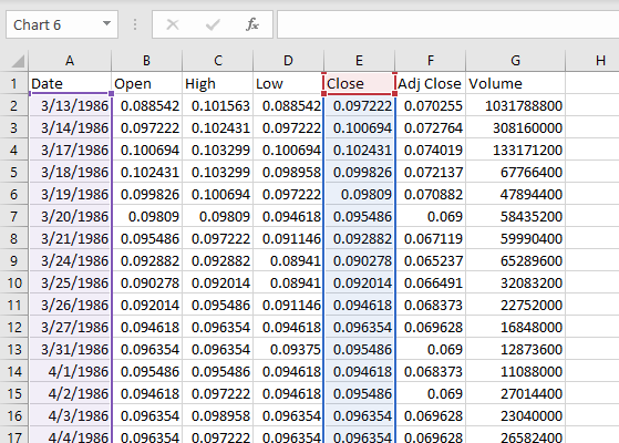
Below is a small sample of the data used to plot this chart. This data can be downloaded from Yahoo Finance .
Steps to create
Create a Line Chart with Date and Close data only.
Remove extra data series, leaving only Date and Close.
Make sure x-axis is formatted as a Date axis.
Set Major units to 5 years, minor units to 1 year.
Set bounds to 1/1/1990 and 1/1/2020.
Apply number format to the axis (“yyyy”) in this case.
Adjust upper bounds for y-axis as desired.
Add a title and apply text formatting as needed
To make a dynamic chart that automatically skips empty values, you can use dynamic named ranges created with formulas. When a new value is added, the chart automatically expands to include the value. If a value is deleted, the chart automatically removes the label.
In the chart shown, data is plotted in one series. Values come from a named range called “values”, defined with the formula provided below:
=$C$4:INDEX($C$4:$C$30,COUNT($C$4:$C$30)) // values
Axis labels come from a named range called “groups”, defined with this formula:
=$B$4:INDEX($B$4:$B$30,COUNT($C$4:$C$30)) // groups
This page explains dynamic named ranges created with INDEX in more detail.
How to make this chart
Create a normal chart, based on the values shown in the table. If you include all rows, Excel will plot empty values as well.
Using the name manager (control + F3) define the name “groups”. In the “refers to” box, use a formula like this:
=$B$4:INDEX($B$4:$B$30,COUNT($C$4:$C$30))
- Define a name for “values” with the same process, using this formula:
=$C$4:INDEX($C$4:$C$30,COUNT($C$4:$C$30))
- Edit the data series with the Select data command. For series values, use the defined name “values” with the sheet name prepended:
=Sheet1!values

For category labels, use the defined name “groups” with the sheet name prepended:
=Sheet1!groups

- Click OK twice to save changes and exit the Select Data dialog.
