Purpose
Return value
Syntax
=LOOKUP(lookup_value,lookup_vector,[result_vector])
- lookup_value - The value to search for.
- lookup_vector - The array or range to search.
- result_vector - [optional] The array or range to return.
Using the LOOKUP function
The LOOKUP function is one of the original lookup functions in Excel. You can use LOOKUP to look up a value in one range or array and return the corresponding value from another range or array. Like the newer XLOOKUP function, LOOKUP can look up values in either rows or columns. However, unlike XLOOKUP, LOOKUP can only perform an approximate match.
LOOKUP has certain default behaviors that make it useful for solving tricky problems in Excel:
- LOOKUP always performs an approximate match.
- LOOKUP assumes that the lookup_vector is sorted in ascending order.
- LOOKUP can look up values in vertical or horizontal ranges/arrays.
- When LOOKUP can’t find an exact match, it matches the next smallest value.
- It can handle some array operations without control + shift + enter (in older versions of Excel).
Here is an example of a traditionally difficult problem that LOOKUP has been able to solve for many years: Get value of last non-empty cell. With the introduction of new power functions like XLOOKUP and XMATCH, LOOKUP is not as important as it was in the past, but if you must use an old version of Excel, LOOKUP can still be quite useful.
The LOOKUP function accepts three arguments: lookup_value, lookup_vector, and result_vector. The first argument, lookup_value, is the value to look for. The second argument, lookup_vector , is the range or array to search. The third argument, result_vector, is the range or array from which to return a result. Result_vector is optional. If result_vector is not provided, LOOKUP returns the value of the match found in lookup_vector . The LOOKUP function has two forms: vector and array. Most of this article describes the vector form, but the last example below explains the array form.
Example #1 - basic usage
In the example shown above, the formula in cell F5 returns the value of the match found in column B. Note that result_vector is not provided:
=LOOKUP(F4,B5:B9) // returns match in level
The formula in cell F6 returns the corresponding Tier value from column C. Notice in this case, both lookup_vector and result_vector are provided:
=LOOKUP(F4,B5:B9,C5:C9) // returns corresponding tier
In both formulas, LOOKUP automatically performs an approximate match, so lookup_vector must be sorted in ascending order.
Example #2 - last non-empty cell
LOOKUP can be used to get the value of the last filled (non-empty) cell in a column. In the screen below, the formula in F6 is:
=LOOKUP(2,1/(B:B<>""),B:B)
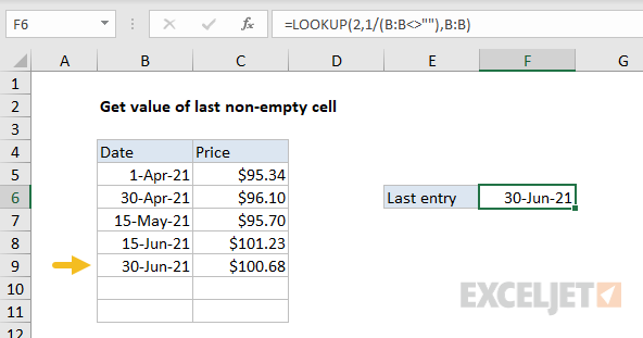
Note the use of a full column reference . This is not an intuitive formula, but it works well. The key to understanding this formula is to recognize that the lookup_value of 2 is deliberately larger than any values that will appear in the lookup_vector . Detailed explanation here .
Example #3 - latest price
Like the above example, the lookup function can be used to look up the latest price in data sorted in ascending order by date. In the screen below, the formula in G5 is:
=LOOKUP(2,1/(item=F5),price)
where item (B5:B12) and price (D5:D12) are named ranges .
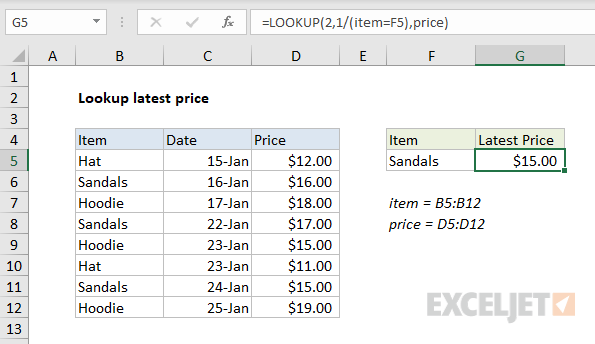
When lookup_value is greater than all values in lookup_array , the default behavior is to “fall back” to the previous value. This formula exploits this behavior by creating an array that contains only 1s and errors, then deliberately looking for the value 2, which will never be found. More details here .
Example #4 - array form
The LOOKUP function has an array form as well. In the array configuration, LOOKUP takes just two arguments: the lookup_value , and a single two-dimensional array:
LOOKUP(lookup_value, array) // array form
In the array form, LOOKUP evaluates the array and automatically changes behavior based on the array dimensions. If the array is wider than tall, LOOKUP looks for the lookup value in the first row of the array (like HLOOKUP ). If the array is taller than wide (or square), LOOKUP looks for the lookup value in the first column (like VLOOKUP ). In either case, LOOKUP returns a value at the same position from the last row or column in the array. The example below shows how the array form works. The formula in F5 is configured to use a vertical array, and the formula in F6 is configured to use a horizontal array:
=LOOKUP(E5,B5:C9) // vertical array
=LOOKUP(E6,C11:G12) // horizontal array
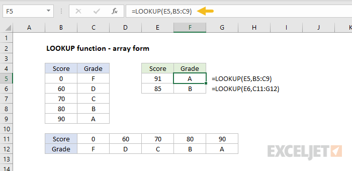
The vertical and horizontal arrays contain the same values; only the orientation is different.
Note: Microsoft discourages the use of the array form and suggests VLOOKUP and HLOOKUP as better options.
Notes
- LOOKUP assumes that lookup_vector is sorted in ascending order.
- When lookup_value can’t be found, LOOKUP will match the next smallest value .
- When lookup_value is greater than all values in lookup_vector , LOOKUP matches the last value.
- When lookup_value is less than the first value in lookup_vector , LOOKUP returns #N/A.
- Result_vector must be the same size as lookup_vector .
- LOOKUP is not case-sensitive
Purpose
Return value
Syntax
=MATCH(lookup_value,lookup_array,[match_type])
- lookup_value - The value to match in lookup_array.
- lookup_array - A range of cells or an array reference.
- match_type - [optional] 1 = exact or next smallest (default), 0 = exact match, -1 = exact or next largest.
Using the MATCH function
The MATCH function is used to determine the position of a value in a range or array . For example, in the screenshot above, the formula in cell E6 is configured to get the position of the value in cell D6. The MATCH function returns 5 because the lookup value (“peach”) is in the 5th position in the range B6:B14:
=MATCH(D6,B6:B14,0) // returns 5
The MATCH function can perform exact and approximate matches and supports wildcards (* ?) for partial matches. There are 3 separate match modes (set by the match_type argument), as described below.
Note: the MATCH function will always return the first match. If you need to return the last match (reverse search) see the XMATCH function . If you want to return all matches, see the FILTER function .
MATCH only supports one-dimensional arrays or ranges , either vertical or horizontal. However, you can use MATCH to locate values in a two-dimensional range or table by giving MATCH the single column (or row) that contains the lookup value. You can even use MATCH twice in a single formula to find a matching row and column at the same time.
Frequently, the MATCH function is combined with the INDEX function to retrieve a value at a certain (matched) position. In other words, MATCH figures out the position , and INDEX returns the value at that position . For a detailed overview with simple examples, see How to use INDEX and MATCH .
Match type information
Match type is optional. If not provided, match_type defaults to 1 (exact or next smallest). When match_type is 1 or -1, it is sometimes referred to as an “approximate match”. However, keep in mind that MATCH will always perform an exact match when possible, as noted in the table below:
| Match type | Behavior | Details |
|---|---|---|
| 1 | Approximate | MATCH finds the largest value less than or equal to the lookup value. The lookup array must be sorted in ascending order. |
| 0 | Exact | MATCH finds the first value equal to the lookup value. The lookup array does not need to be sorted. |
| -1 | Approximate | MATCH finds the smallest value greater than or equal to the lookup value. The lookup array must be sorted in descending order. |
| (omitted) | Approximate | When match_type is omitted, it defaults to 1 with behavior as explained above. |
Caution: Be sure to set match_type to zero (0) if you need an exact match. The default setting of 1 can cause MATCH to return results that look normal but are in fact incorrect. Explicitly providing a value for match_type, is a good reminder of what behavior is expected.
Exact match
When match_type is zero (0), MATCH performs an exact match only. In the example below, the formula in E3 is:
=MATCH(E2,B3:B11,0) // returns 4

In the formula above, the lookup value comes from cell E2. If the lookup value is hardcoded into the formula, it must be enclosed in double quotes (""), since it is a text value:
=MATCH("Mars",B3:B11,0)
Note: MATCH is not case-sensitive, so “Mars” and “mars” will both return 4.
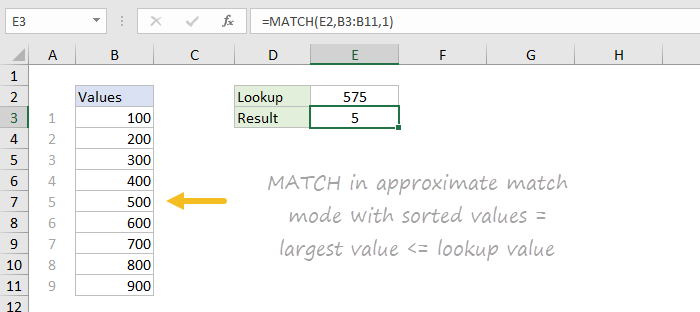
Approximate match
When match_type is set to 1, MATCH will perform an approximate match on values sorted A-Z, finding the largest value less than or equal to the lookup value. In the example shown below, the formula in E3 is:
=MATCH(E2,B3:B11,1) // returns 5
Wildcard match
When match_type is set to zero (0), MATCH can use wildcards . In the example shown below, the formula in E3 is:
=MATCH(E2,B3:B11,0) // returns 6
This is equivalent to:
=MATCH("pq*",B3:B11,0)

INDEX and MATCH
The MATCH function is commonly used together with the INDEX function . The resulting formula is called “INDEX and MATCH”. For example, in the screen below, INDEX and MATCH are used to return the cost of a code entered in cell F4. The formula in F5 is:
=INDEX(C5:C12,MATCH(F4,B5:B12,0)) // returns 150
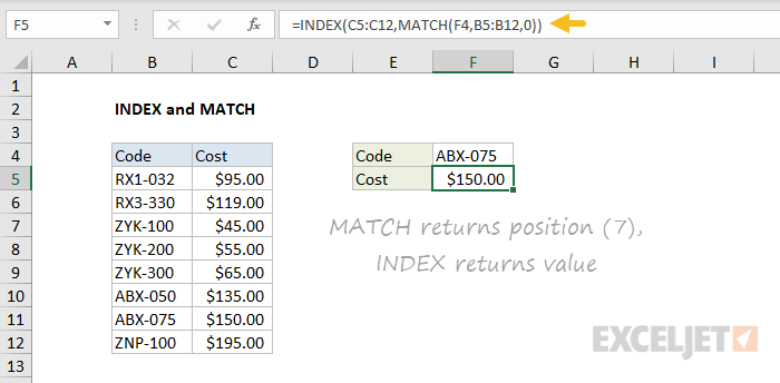
In this example, MATCH is set up to perform an exact match. The MATCH function locates the code ABX-075 and returns its position (7) directly to the INDEX function as the row number. The INDEX function then returns the 7th value from the range C5:C12 as a final result. The formula is solved like this:
=INDEX(C5:C12,MATCH(F4,B5:B12,0))
=INDEX(C5:C12,7)
=150
See below for more examples of the MATCH function. For an overview of how to use INDEX and MATCH with many examples, see: How to use INDEX and MATCH .
Case-sensitive match
The MATCH function is not case-sensitive. However, MATCH can be configured to perform a case-sensitive match when combined with the EXACT function in a generic formula like this:
=MATCH(TRUE,EXACT(lookup_value,array),0)
The EXACT function compares every value in array with the lookup_value in a case-sensitive manner. This formula is explained with an INDEX and MATCH example here .
Notes
- MATCH is not case-sensitive.
- MATCH returns the #N/A error if no match is found.
- MATCH only works with text up to 255 characters in length.
- In case of duplicates, MATCH returns the first match.
- If match_type is -1 or 1, the lookup_array must be sorted as noted above.
- If match_type is 0, the lookup_value can contain the wildcards .
- The MATCH function is frequently used together with the INDEX function .
