Explanation
In this example, the goal is to make a noun plural when the number of items is greater than one. In many cases, a noun can be made plural by adding an “s”. However, many nouns have an irregular plural form, and the main challenge is to handle these exceptions.
Ingredients
In the example shown, the formula uses these ingredients:
- IF function – to check the number of items
- VLOOKUP function – to lookup irregular plural forms
- IFNA function – to take action when there is no irregular form
- Concatenation – to glue text together
Note: There are many ways to solve a problem like this in Excel, and this is just one approach.
Adding an “s”
In the simplest case, the only task is to add an “s” to the end of a word using concatenation . This can be done with a formula like this:
=C5&"s" // simple concatenation
The ampersand operator (&) is used to join an “s” to the word in column C.
However, we don’t want to add an “s” unless the number in column B is greater than 1. For this, we can use the IF function to check the number in column B:
=IF(B5>1,C5&"s"),C5)
In this version of the formula, we only add an “s” when the number in B5 is greater than 1. At this point, the formula handles the base case without trouble, but it won’t handle words with irregular plural forms.
Handling irregular forms
To handle words with an irregular plural form, we need to perform a lookup. In the example shown, we do this with the VLOOKUP function :
=VLOOKUP(C5,wordtable,2,0)
where wordtable is the named range F5:G11. Here, we use VLOOKUP to locate a word in a table and return the irregular plural from the second column. Obviously, this only works when the table contains an entry for a given word. If a word does not exist in the table, VLOOKUP will return a #N/A error, and we can use this error to take some other action. The trick is to nest VLOOKUP inside the IFNA function to trap the error like this:
=IFNA(VLOOKUP(C5,wordtable,2,0),other)
where “other” represents a different action. The idea is that words with an irregular plural form need to have an entry in the table. At this point in the formula, we know the word should be plural. If we check the table and can’t find the word, we can assume the word does not have an irregular plural form and we can simply add an “s”.
Putting it all together
We now have all the pieces we need for a single formula:
- Make plural only when number > 1
- Handle a regular plural form
- Handle an irregular plural form
We now need to assemble these pieces together in a logical flow like this:
If number is greater than one, make the word plural, otherwise, return the original word. When making a word plural, check a custom table first to see if there is an irregular form. If there is an irregular form, use it. If an entry is not found, simply add an “s”.
The formula that implements this logic looks like this:
IF(B5>1,IFNA(VLOOKUP(C5,wordtable,2,0),C5&"s"),C5)
The formula that appears in the example performs one additional step: it concatenates the number from column B to the result from the formula above so that the number appears together with the plural form of the noun:
=B5&" "&IF(B5>1,IFNA(VLOOKUP(C5,wordtable,2,0),C5&"s"),C5)
This results in a text string like “3 apples” and it makes it easier to quickly check results.
Note: if a noun has an irregular form but is not listed in the custom table, this formula will incorrectly add an “s”. Therefore, all words with an irregular plural form that you want to handle must exist in the custom table. This is a limitation of the formula.
Explanation
In this example, the goal is to return the most frequently occurring text based on one or more supplied criteria. Working from the inside out, we use the MATCH function to match the text range against itself, by giving MATCH the same range for lookup value and lookup array, with zero for match type:
MATCH(supplier,supplier,0)
Since the lookup value is an array with 10 values, MATCH returns an array of 10 results:
{1;1;3;3;5;1;7;3;1;5;5}
Each item in this array represents the first position at which a supplier name appears in the data. This array is fed into the IF function , which is used to filter results for Client A only:
IF(client=F5,{1;1;3;3;5;1;7;3;1;5;5})
IF returns the filtered array to the MODE function :
{1;FALSE;3;FALSE;5;1;FALSE;FALSE;1;5;FALSE}
Notice only positions associated with Client A remain in the array. MODE ignores FALSE values and returns the most frequently occurring number to the INDEX function as the row number:
=INDEX(supplier,1)
Finally, with the named range “supplier” as the array, INDEX returns “Brown”, the most frequently occurring supplier for Client A.
Mode of text from every other row
Following the example above, the formula below has been adapted to return the most frequent text from every other row. The formulas in E5 and E6 are:
=INDEX(text,MODE(IF(MOD(ROW(text),2)=1,MATCH(text,text,0)))) // odd
=INDEX(text,MODE(IF(MOD(ROW(text),2)=0,MATCH(text,text,0)))) // even
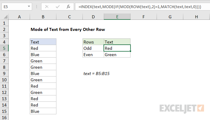
The overall structure of the formulas above is the same as the original example above. The key difference is the logical test used to check even and odd rows with the named range text (B5:B15). Both formulas use the MOD function with a divisor of 2:
MOD(ROW(text),2)=1 // check for odd
MOD(ROW(text),2)=0 // check for even
If the remainder is 1, we have an odd row. If the remainder is 0 (zero), we have an even row. These tests act as a filter for incoming text so that the result from the first formula is the most frequently occurring text in odd rows, and the result from the second formula is the most frequently occurring text in even rows.
