Explanation
In the example shown, the goal is to calculate the maximum difference between the “High” values in column C and the “Low” values in column D. Because the difference between High and Low is not part of the data, the calculation must occur in the formula itself. This is a classic example of an array formula .
Excel Table
For convenience, all data is in an Excel Table named data in the range B5:D16. Excel Tables are a convenient way to work with data in Excel because they (1) automatically expand to include new data and (2) offer structured references , which let you refer to data by name instead of by address. If you are new to Excel Tables, this article provides an overview . Also, see this short video:
Video: How to create an Excel Table
Array formula
This is a classic array formula problem. Subtracting the lows from the highs is an array operation that requires special handling in older versions of Excel. In Legacy Excel, you must enter the formula with control + shift + enter. When you enter the formula this way, you will see the formula enclosed in curly braces like this:
{=MAX(data[High]-data[Low])}
Note: This is an array formula and must be entered with control + shift + enter in Legacy Excel. If you open the workbook in an older version of Excel you will see that Excel automatically adds the curly braces. This is done to make sure the formula works properly. If you re-enter the formula without control + shift + enter, you will see an incorrect result. In the current version of Excel, you will not see the curly braces, and it is not necessary to enter the formula in a special way.
Video: What is an array formula?
Maximum change
To calculate the maximum change, the formula in cell F5 is:
=MAX(data[High]-data[Low])
After the table references are evaluated, we have the high and low values in array form:
=MAX({79;77;76;69;72;76;79;83;85;79;82;83}-{68;69;64;55;59;60;64;69;62;60;73;76})
After subtraction, we have a single array inside the MAX function. The values in this array represent change:
=MAX({11;8;12;14;13;16;15;14;23;19;9;7})
The MAX function returns 23, the maximum change between high and low in this set of data.
Minimum change
To return the minimum change, replace the MAX function with the MIN function :
=MIN(data[High]-data[Low])
Absolute change
In the table shown, the high values are always greater than the low values, which means the change itself will be a positive number. If you are comparing two columns of data where that is not true, the change will sometimes be negative. If you want to ignore the negative sign, you can add the ABS function to the formula like this:
=MAX(ABS(data[High]-data[Low]))
The ABS function returns the absolute value of a number, so it will convert any negative numbers to positive numbers. The MAX function will then return the maximum absolute value change.
Date of max change
You may also want to know the date of the maximum change. In the worksheet shown, cell G5 contains an INDEX and MATCH formula to return the date associated with the max change:
=INDEX(data[Date],MATCH(F5,data[High]-data[Low],0))
Note: This is an array formula and must be entered with control + shift + enter in Legacy Excel.
The gist of this formula is that we are using the maximum change value like a “key” to locate the date. Most of the work is done in the MATCH function , which calculates the matching row number like this:
=MATCH(F5,data[High]-data[Low],0)
=MATCH(23,{11;8;12;14;13;16;15;14;23;19;9;7},0)
=9
Note that we run the same change calculation explained above inside MATCH as the lookup_array . Then we match the value in cell F5 against all changes in lookup_array , which we know contains the max change. MATCH returns 9 to INDEX as row_num , and INDEX returns June 9 as a final result.
=INDEX(data[Date],9) // returns 9-Jun
Note: if the change values contain duplicates, MATCH will match the first occurrence and INDEX will return the date of the first occurrence.
XLOOKUP
If your version of Excel has XLOOKUP, you can write a more compact version of the date lookup like this:
=XLOOKUP(F5,data[High]-data[Low],data[Date])
The logic is the same as with INDEX and MATCH: we look for the max change in F5 inside an array of calculated changes and return the corresponding date. In addition to offering a more streamlined formula, the XLOOKUP function gives you controls to return the first or last match .
All in one formula
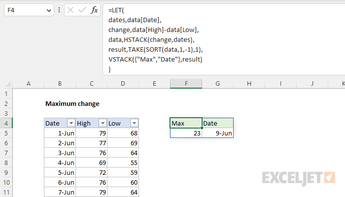
In the dynamic array version of Excel , you can use a formula that creates the entire table in one step:
=LET(
dates,data[Date],
change,data[High]-data[Low],
data,HSTACK(change,dates),
result,TAKE(SORT(data,1,-1),1),
VSTACK({"Max","Date"},result)
)
The screen below shows what this formula looks like in the worksheet:
We use the LET function to assign values to four variables: dates , change , data , and result . The values for dates come from the Date column directly:
=LET(
dates,data[Date],
The values for change come from the change calculation explained above:
=LET(
dates,data[Date],
change,data[High]-data[Low],
Next, we assemble the two columns we want in the final result using the HSTACK function to join change to dates :
=LET(
dates,data[Date],
change,data[High]-data[Low],
data,HSTACK(change,dates),
This creates a two-column array with change values in the first column and date values in the second column. The result is assigned to data . Next, we assign a value to the result using SORT and TAKE:
=LET(
dates,data[Date],
change,data[High]-data[Low],
data,HSTACK(change,dates),
result,TAKE(SORT(data,1,-1),1),
Inside TAKE, we use the SORT function to sort data by the first column in descending order. Then we use the TAKE function to retrieve just the first row, which (because we sorted in descending order by change) contains the maximum change and date of maximum change. Last, we assemble our table with the VSTACK function , which returns a final result:
=LET(
dates,data[Date],
change,data[High]-data[Low],
data,HSTACK(change,dates),
result,TAKE(SORT(data,1,-1),1),
VSTACK({"Max","Date"},result)
)
The result is the entire table shown in the range F4:G5.
Notes:
- To return the nth largest values, change the 2nd argument in TAKE to n. For example, to return the top 3 changes, you can ask TAKE for 3 rows instead of 1 row.
- To return the minimum change, change the 3rd argument in SORT to 1 to sort in ascending order
Explanation
In this example, the goal is to get the maximum value for a given group below a specific temperature. In other words, we want the max value after applying multiple criteria. The easiest way to solve this problem is with the MAXIFS function. However, if you need more flexibility (i.e., you need to work with arrays and not ranges), you can use the MAX function with the FILTER function. In older versions of Excel without MAXIFS or FILTER, you can use a traditional array formula based on the MAX function and the IF function. Each approach is explained below.
Excel Table
For convenience, all data is in an Excel Table named data in the range B5:D16. Excel Tables are a convenient way to work with data in Excel because they (1) automatically expand to include new data and (2) offer structured references , which allow you to refer to data by name instead of by address. If you are new to Excel Tables, this article provides an overview .
Video: How to create an Excel Table
MAXIFS function
One way to solve this problem is with the MAXIFS functio n, which can get the maximum value in a range based on one or more criteria. The generic syntax for MAXIFS with two conditions looks like this:
=MAXIFS(max_range,range1,criteria1,range2,criteria2)
Note that each condition is defined by two arguments : range1 and criteria1 define the first condition, and range2 and criteria2 define the second condition. All conditions must be true in order for the value to be considered. We start off with the max_range , which is the Value column in the table:
=MAXIFS(data[Value],
Next, we add criteria to test for the group value entered in cell F5:
=MAXIFS(data[Value],data[Group],F5
If we enter the formula above as-is, we will get the maximum value in group “A”. Next, we need to add a second condition to further restrict values below the temperature entered in cell G5:
=MAXIFS(data[Value],data[Group],F5,data[Temp],"<"&G5)
Notice we need to concatenate the less than operator ("<") to cell F5. This is a requirement of the MAXIFS function, which uses an unusual formula syntax shared by SUMIFS, COUNTIFS, etc. When we enter this formula, it returns the maximum value in group “A” below a temperature of 73. For reference, the same formula with conditions hardcoded looks like this:
=MAXIFS(data[Value],data[Group],"A",data[Temp],"<73")
MAXIFS will automatically ignore empty cells that meet the criteria. In other words, MAXIFS will not treat empty cells that meet the criteria as zero. On the other hand, MAXIFS will return zero (0) if no cells match the given criteria.
The MAXIFS function works well, but it does have one significant limitation: the range arguments inside MAXIFS must be actual ranges , you can’t substitute arrays . If you need to use arrays, see the MAX + FILTER option below.
MAX + FILTER
In the dynamic array version of Excel , another way to solve this problem is with MAX and FILTER, like this:
=MAX(FILTER(data[Value],(data[Group]=F5)*(data[Temp]<G5)))
Inside the MAX function, the FILTER function is configured to filter values by group and temperature:
FILTER(data[Value],(data[Group]=F5)*(data[Temp]<G5))
Array is provided as the Value column in the table. The include argument is a simple expression:
(data[Group]=F5)*(data[Temp]<G5)
This is an example of using Boolean logic in Excel. Because there are 12 values in the table, each expression above generates an array of 12 TRUE and FALSE values like this:
{TRUE;FALSE;FALSE;TRUE;FALSE;FALSE;TRUE;FALSE;FALSE;TRUE;FALSE;FALSE}*{TRUE;TRUE;TRUE;TRUE;TRUE;TRUE;FALSE;FALSE;FALSE;FALSE;FALSE;FALSE}
The math operation of multiplication (*) converts the TRUE and FALSE values to 1s and 0s:
{1;0;0;1;0;0;1;0;0;1;0;0}*{1;1;1;1;1;1;0;0;0;0;0;0}
And the result is a single array as the include argument, like this:
FILTER(data[Value],{1;0;0;1;0;0;0;0;0;0;0;0})
Note that the 1s in this array correspond to values that are in group “A” with a temperature below 73. FILTER returns the two values that meet these criteria directly to the MAX function:
=MAX({83;88})
And MAX returns 88 as a final result. The primary advantage of using the MAX function with the FILTER function is that you don’t need to provide a range of values on the worksheet. You can instead provide an array of values created with another operation. This is important when source data needs to be manipulated before a max value is calculated.
MAX + IF
In older versions of Excel that do not have the MAXIFS function or the FILTER function, you can solve this problem with an array formula based on the MAX function and the IF function, like this:
=MAX(IF((data[Group]=F5)*(data[Temp]<G5),data[Value]))
Note: This is an array formula and must be entered with control + shift + enter in Legacy Excel .
Working from the inside out, the IF function is evaluated first. The logical test inside IF is exactly the same as the logic explained above for FILTER:
(data[Group]=F5)*(data[Temp]<G5) // logical test
After the logic is evaluated, we have an array of 1s and 0s like this:
=MAX(IF({1;0;0;1;0;0;0;0;0;0;0;0},data[Value]))
The 1s correspond to rows where the group is “A” and the temperature is less than 73. The final result from IF is an array like this:
{83;FALSE;FALSE;88;FALSE;FALSE;FALSE;FALSE;FALSE;FALSE;FALSE;FALSE}
Looking at the values in this array, you can see that the IF function acts like a filter: only values associated with group “A” and a temperature less than 73 make it through the filter. The other values are replaced with FALSE. The IF function delivers this array directly to the MAX function :
=MAX({83;FALSE;FALSE;88;FALSE;FALSE;FALSE;FALSE;FALSE;FALSE;FALSE;FALSE})
The MAX function automatically ignores FALSE values and returns the maximum number in the array: 88.
Alternative syntax with nested IFs
The array formula above uses Boolean logic to streamline the formula, but another option you might run into is nesting one IF formula inside another, like this:
=MAX(IF(data[Group]=F5,IF(data[Temp]<G5,data[Value])))
Note: This is an array formula and must be entered with control + shift + enter in Legacy Excel .
Each IF formula applies a separate condition, so the values are filtered in two steps instead of one. This works fine, but the formula gets more complicated as additional criteria are added, since each condition requires another IF function. The advantage Boolean logic version of the formula is that you can add additional criteria without adding more IF functions.
