- What is the 4% retirement rule?
- How the 4% rule works
- What we need to model in Excel
- The model in Excel
- Traditional approach (Sheet1)
- Hybrid approach (Sheet2)
- Single formula approach (Sheet3)
- Summary and conclusion
- Functions used in the workbook
- Instructions
What is the 4% retirement rule?
If you look into retirement planning, you’ll probably run into the 4% retirement rule, one of the most well-known (and frequently cited) guidelines for retirement spending. In brief, the 4% retirement rule tries to answer this question in a simple way: “How much can I safely withdraw from my retirement savings each year without running out of money?” The answer? About 4%, adjusted for inflation.
The rule came out of research conducted by a financial advisor named Bill Bengen in 1994. His goal was to determine a safe withdrawal rate (SAFEMAX) that would allow retirees to maintain their standard of living throughout a 30-year retirement without running out of money, even across periods of poor market performance and high inflation.
Based on a historical reconstruction of retiree portfolios since 1926, Bengen recommended a 4% withdrawal rate for the first year, followed by cost-of-living adjustments each succeeding year. Although Bengen himself didn’t refer to a “4% rule” (and later changed his recommendation to 4.5% and then to 4.7%), the name stuck and carries on to this day.
How the 4% rule works
Applying the rule is simple: in your first year of retirement, you withdraw 4% of your total portfolio balance. In each subsequent year, you adjust that initial dollar amount for inflation rather than recalculating 4% of your current balance. For example, if you retire with a $1 million portfolio, you would withdraw $40,000 in year one. If inflation is 3% that year, you’d withdraw $41,200 in year two, and so on. The idea is to provide predictable, inflation-adjusted income while preserving the portfolio across various market conditions across the entire retirement period.
For those planning retirement, the 4% rule serves as both a withdrawal strategy and a savings target. If you know your desired annual retirement income, you can work backward to determine how much you need to save: simply multiply your target income by 25 (since 4% × 25 = 100%). While the rule has plenty of critics and may need adjustment based on individual circumstances, it remains a useful starting point for retirement planning. It is also a great example of a problem that can be modeled in Excel, where you can easily test various scenarios and assumptions.
I’m not a financial advisor. My goal is not to convince you that the 4% rule is the best way to plan for retirement. My goal is to show how you can model a problem like this in Excel in different ways.
What we need to model in Excel
Before we get into details, let’s review what we need to model: Beginning with a given starting balance (total retirement savings), we need to calculate 4% of the starting balance, then adjust the withdrawal for inflation annually, add in growth and show how this plays out over 30 years. We’ll want inputs for starting balance, withdrawal rate, growth rate, inflation rate, age at retirement, and the number of years in retirement, so that we can fiddle with these numbers to see how they impact the final outcome:
| Input | Description | Example value |
|---|---|---|
| Starting balance | Total retirement savings at the beginning | $1,000,000 |
| Withdrawal rate | Initial withdrawal percentage | 4% |
| Annual growth rate | Expected portfolio return | 7% |
| Inflation rate | Annual cost-of-living increase | 2.5% |
| Age at retirement | Starting age | 65 |
| Years in retirement | Duration of withdrawal period | 30 |
In our Excel model, we’ll use constant rates for both growth and inflation throughout the entire retirement period. This is a simplification that makes the model easier to build and understand. In reality, portfolio returns vary significantly from year to year (i.e. gains of 20% on year, others losses of 15% in another) and you would adjust withdrawals based on actual annual inflation rather than an assumed rate. The sequence of these returns matters a lot: poor market performance early in retirement is far more damaging than the same poor returns later on. This is called “sequence of returns risk,” and it’s why Bengen tested his 4% rule against historical market data, including worst-case scenarios like retiring in 1968 just before a major market decline and high inflation period. Our constant-rate model won’t capture this real-world volatility, but it will demonstrate the mechanics of how the 4% rule works.
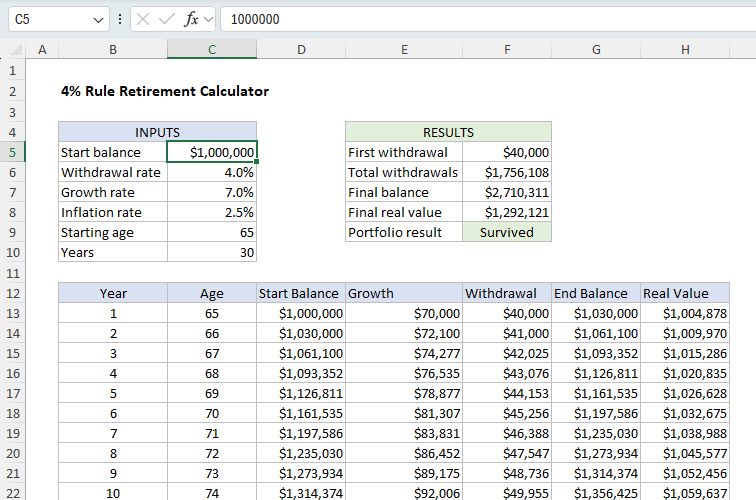
Using the inputs above, we need to generate a “withdrawal schedule” that shows how the portfolio changes over a period of 30 years. Once we have the schedule in place, we can calculate the total withdrawals and a final balance to see if the portfolio survived retirement. We also want to calculate a “real value” of the ending balance, adjusted for inflation. Finally, we want the withdrawal schedule to be dynamic, so that it expands or contracts as needed when the number of years in retirement changes. The screenshot below shows the basic idea. Note the key inputs are in the range C5:C10. These are the variables that control the outputs. The outputs are summarized in the range F5:F9. The withdrawal schedule begins in row 13 and covers 30 years.
The model in Excel
Of course, there are different ways to model a problem like this in Excel, especially since Excel now supports dynamic array formulas , which offer entirely new ways to approach multi-row calculations. The attached workbook explores three different ways to model the 4% retirement rule. All approaches use the same inputs and produce identical outputs, but they build the withdrawal schedule in progressively more advanced ways — from classic formulas to modern dynamic arrays.
- Sheet1 - Traditional approach - Classic row-by-row formulas with relative and absolute references.
- Sheet2 - Hybrid approach - One dynamic array formula per column.
- Sheet3 - Single formula approach - One formula generates the entire table.
The workbook also has a fourth sheet with simple instructions on how to use the workbook.
The point of this exercise is not to convince you that one approach is better than the other. The point is to look at different ways to model a problem like this in Excel, and explore some of the pros and cons of each approach. Let’s start with the traditional approach.
As shipped, all three worksheets have the same inputs and produce the same outputs. The only difference is the approach used to build the withdrawal schedule and the summary results in column F. On any sheet, you can modify the inputs in the range C5:C10 to see how the outputs change. The changes you make on one sheet will not affect the other sheets.
Traditional formula approach (Sheet1)
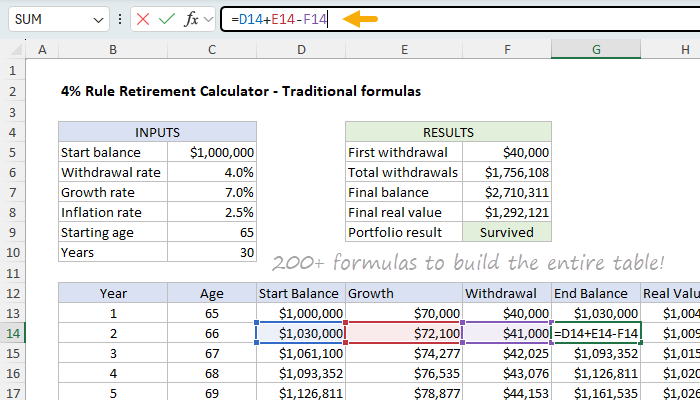
This worksheet uses a classic row-by-row setup — each row represents one year of retirement, and every column holds a key variable: Year, Age, Start Balance, Growth, Withdrawal, End Balance, and Real Value (inflation-adjusted balance). Formulas are copied down and use a mix of relative and absolute references so that each row refers correctly to the previous year’s results. It takes more than 200 formulas to build the entire withdrawal schedule for 30 years.
Here is how the formulas are set up:
| Column | Description | Example formula (first data row) |
|---|---|---|
| B - Year | Sequence of years | 1 in row 13, then B13+1 |
| C - Age | Age in each year | =C9 in row 13, then C13+1 |
| D - Start Balance | Beginning portfolio value | =C5 in row 13, then G13 |
| E - Growth | Portfolio growth | =D13*$C$7 |
| F - Withdrawal | Inflation-adjusted withdrawal | =C5C6 in row 13, then =F13(1+$C$8) |
| G - End Balance | End of year balance | =D13+E13-F13 |
| H - Real Value | Inflation-adjusted end balance | =PV($C$8,B13,0,-G13) |
The summary results in the range F5:F9 are generated with the following formulas:
| Cell | Description | Formula |
|---|---|---|
| F5 | First withdrawal | =C5*C6 |
| F6 | Total withdrawals | =SUM(F13:F100) |
| F7 | Final balance | =LOOKUP(2,1/(G13:G100<>""),G13:G100) |
| F8 | Total real value | =LOOKUP(2,1/(H13:H100<>""),H13:H100) |
| F9 | Portfolio result | =IF(F7>0,“Survived”,“Depleted”) |
The LOOKUP function is used to find the last non-empty cell in the range G13:G100 and H13:H100. These ranges are oversized to allow the table to be extended if needed. For more details on this formula see Get value of last non-empty cell . The LOOKUP function works in all Excel versions. You could use the same trick to pull the last year in column B into C10 (Years) if you like, but I have left it as a static value to avoid confusion. For more information on the PV function, see PV function .
Note that a key feature of this approach is that formulas in row 1 of the schedule are often different from the formulas in the subsequent rows. These formulas must be carefully crafted to ensure that they reference the correct cells, which involves using a mix of relative and absolute references. It also means a user must be careful if changes are made to the withdrawal schedule. On the other hand, this approach is easy to understand and audit, and works in all Excel versions.
Pros and cons
| Pros | Cons |
|---|---|
| Easy to understand and audit | Must copy or extend formulas manually |
| Works in all Excel versions | Fixed size, table is not dynamic |
| Great for teaching relative/absolute references | Prone to reference errors if rows are inserted or deleted |
Hybrid formula approach (Sheet2)
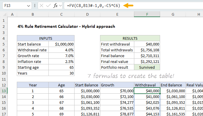
This sheet uses dynamic array formulas to generate each full column of data automatically. Every column uses one formula that spills to the required number of rows, tied initially to the Years (C10) input. It takes 7 formulas to build the entire withdrawal schedule, one per column:
The formulas are set up like this:
| Column | Description | Formula |
|---|---|---|
| B - Year | Sequence of years | =SEQUENCE(C10) |
| C - Age | Starting age + sequence | =SEQUENCE(C10,1,C9) |
| D - Start Balance | Prior year’s end | =VSTACK(C5,DROP(G13#,-1)) |
| E - Growth | Annual growth | =D13#*C7 |
| F - Withdrawal | Inflation-adjusted withdrawal | =FV(C8,B13#-1,0,-C5*C6) |
| G - End Balance | Balance after growth and withdrawal | =SCAN(C5,F13#,LAMBDA(bal,wd,bal*(1+C7)-wd)) |
| H - Real Value | Inflation-adjusted balance | =PV(C8,B13#,0,-G13#) |
The summary results in the range F5:F9 are generated with the following formulas:
| Cell | Description | Formula |
|---|---|---|
| F5 | First withdrawal | =C5*C6 |
| F6 | Total withdrawals | =SUM(F13#) |
| F7 | Final balance | =TAKE(G13#,-1) |
| F8 | Total real value | =TAKE(H13#,-1) |
| F9 | Portfolio result | =IF(F7>0,“Survived”,“Depleted”) |
This approach in Sheet2 is a great example of how formulas can be anchored to an existing spill range so that columns automatically expand or contract as needed. All the formulas in columns D through H are anchored to a spill range for years that begins in cell B13, so that they automatically adjust to the correct number of rows as needed. The spill range for years is generated with the SEQUENCE function like this:
=SEQUENCE(C10) // generate years 1 to 30
If the number of years in cell C10 is changed, the rows in the Year column will expand or contract as needed. Column C (Age) is also created with the SEQUENCE function, which is configured to generate a sequence of ages that spans the same number of years as the Year column, beginning at the starting age in cell C9, and increasing by 1 for each year.
=SEQUENCE(C10,1,C9) // generate ages 65 to 94
Column D (Start Balance) is generated with a clever combination of the DROP and VSTACK functions, like this:
=VSTACK(C5,DROP(G13#,-1))
DROP removes the last (unused) year-end balance from the spill range in column G (End Balance). VSTACK then inserts the starting balance in C5 at the top of the list and appends the year-end balance. It is a bit confusing that the start balance comes before the end balance, and yet the start balance depends on the end balance. But it makes sense if you think about it - the start balance is really the same as the end balance shifted down by one year. In other words, we need the end balance to know the starting balance in the next year.
Column E (Growth) is generated by multiplying the start balance by the growth rate:
=D13#*C7
Column F (Withdrawal) is generated by the FV function . The FV function calculates the future value of an investment based on an initial principal balance, a fixed annual interest rate, the number of compounding periods, and the periodic payment. In this case, we are using the FV function to calculate the future value of the initial withdrawal amount, adjusted for inflation, over the number of years in the withdrawal schedule. The formula looks like this:
=FV(C8,B13#-1,0,-C5*C6)
The rate is supplied as the inflation rate in C8 (2.5%), the number of periods is the number of years in the withdrawal schedule minus 1 B13#-1 , the present value is the starting balance multiplied by the withdrawal rate -C5*C6 , and the payment is 0 since there are no periodic payments.
We use the FV function here to calculate an inflation-adjusted withdrawal, but we could use the equivalent long-hand formula: =C5C6(1+C8)^(B13#-1) . Both formulas will return the same result.
Column G (End Balance) is generated by the SCAN function . The SCAN function applies a LAMBDA function to a series of values and accumulates the results. In this case, we are using the SCAN function to calculate the year-end balances by applying the LAMBDA function to the starting balance and the withdrawal. The formula looks like this:
=SCAN(C5,F13#,LAMBDA(bal,wd,bal*(1+C7)-wd))
The starting balance is supplied as the starting value in C5 , the series of values is the series of withdrawals in F13# , and the LAMBDA function is LAMBDA(bal,wd,bal*(1+C7)-wd) . The LAMBDA function is applied to the starting value and the first value in the series, and the result is returned. The result is then used as the starting value for the next iteration of the LAMBDA function. This process is repeated for each value in the series. With 30 years in C10, the result is a series of 30 year-end balances.
Column H (Real Value) is generated by the PV function . The PV function calculates the present value of an investment based on a future value, a fixed annual interest rate, the number of compounding periods, and the periodic payment. In this case, we are using the PV function to calculate the present value of the year-end balances, adjusted for inflation. The formula looks like this:
=PV(C8,B13#,0,-G13#)
The rate is supplied as the inflation rate in C8 (2.5%), the number of periods is the number of years in the withdrawal schedule B13# , the future value is the year-end balances in G13# , and the payment is 0 since there are no periodic payments.
We use the PV function here to calculate an inflation-adjusted end balance, but we could use the equivalent long-hand formula: =G13#/(1+$C$8)^(B13#) . Both formulas will return the same result.
As mentioned above, because these formulas are tied to the spill ranges, beginning with the spill range in column B (Year), all columns will resize as needed if the number of years in retirement C10 is changed.
Excel’s PV and FV functions use a cash flow convention where you negate values that represent outflows. This is why the present value is negative in the FV function and the future value is positive in the PV function. The negative sign ensures that we get a positive result.
Pros and cons
| Pros | Cons |
|---|---|
| Fully dynamic — table resizes automatically | Requires Excel 365 |
| One formula per column, no locked references | Depends on anchoring to spill ranges |
| Clean, scalable, and easy to read | New functions like SCAN and VSTACK may be unfamiliar |
| Fewer formulas to manage | More abstract than row-by-row approach |
Single formula approach (Sheet3)
In this sheet, the entire withdrawal schedule is generated by a single dynamic array formula that combines LET, SEQUENCE, FV, SCAN, VSTACK, and HSTACK. Each variable is defined and reused inside a single expression, which spills into a complete table. It takes 9 formulas to build the entire withdrawal schedule:
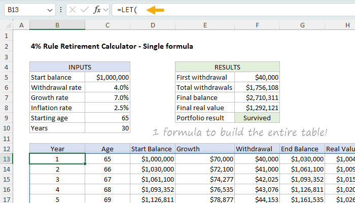
The formula in B13 looks like this:
=LET(
  start,C5, wr,C6, gr,C7, ir,C8, age,C9, n,C10,
  yrs,SEQUENCE(n),
  ages,SEQUENCE(n,1,age),
  wds,FV(ir,yrs-1,0,-start*wr),
  ends,SCAN(start, wds, LAMBDA(bal,wd, bal*(1+gr)-wd)),
  starts,VSTACK(start,DROP(ends,-1)),
  growth,starts*gr,
  real,PV(ir,yrs,0,-ends),
  HSTACK(yrs,ages,starts,growth,wds,ends,real)
)
This formula uses the LET function to define a series of variables that are used to generate the withdrawal schedule:
| Variable | Description |
|---|---|
| start | Starting portfolio balance from C5 ($1,000,000) |
| wr | Withdrawal rate from C6 (4%) |
| gr | Annual growth rate from C7 (7%) |
| ir | Inflation rate from C8 (2.5%) |
| age | Starting age from C9 (65) |
| n | Number of years from C10 (30) |
| yrs | Sequence of years 1 to n |
| ages | Sequence of ages starting at age |
| wds | Annual withdrawals, adjusted for inflation via FV function |
| ends | Year-end balances generated by SCAN |
| starts | Start balances built from prior year’s end |
| growth | Annual growth amounts from start balance * growth rate |
| real | Inflation-adjusted end balances via PV function |
The summary results in the range F5:F9 are generated with the following formulas:
| Cell | Description | Formula |
|---|---|---|
| F5 | First withdrawal | =C5*C6 |
| F6 | Total withdrawals | =SUM(CHOOSECOLS(B13#,5)) |
| F7 | Final balance | =TAKE(CHOOSECOLS(B13#,6),-1) |
| F8 | Total real value | =TAKE(CHOOSECOLS(B13#,7),-1) |
| F9 | Portfolio result | =IF(F7>0,“Survived”,“Depleted”) |
This is clearly the most complex formula of the three approaches, but it is also the most compact and efficient. One nice feature of building the formula this way is that once the variables are defined, they can be used directly in other parts of the formula instead of cell references, making the formula easier to read and understand. Briefly, the formula works like this:
- Define the starting balance (start), withdrawal rate (wr), growth rate (gr), inflation rate (ir), starting age (age), and number of years (n). start,C5, wr,C6, gr,C7, ir,C8, age,C9, n,C10
- Generate a sequence of years (yrs) from 1 to n. yrs,SEQUENCE(n)
- Generate a sequence of ages (ages) starting at the starting age. ages,SEQUENCE(n,1,age)
- Generate a series of annual withdrawals (wds), adjusted for inflation via the FV function . wds,FV(ir,yrs-1,0,-start*wr)
- Generate a series of year-end balances (ends) by applying the SCAN function to the starting balance and the series of annual withdrawals. ends,SCAN(start, wds, LAMBDA(bal,wd, bal*(1+gr)-wd))
- Generate a series of start balances (starts) by building from the prior year’s end. starts,VSTACK(start,DROP(ends,-1))
- Generate a series of annual growth amounts (growth) by multiplying the start balance by the growth rate. growth,starts*gr
- Generate a series of inflation-adjusted end balances (real) by applying the PV function to the year-end balances. real,PV(ir,yrs,0,-ends)
- Combine all the series into a single table using the HSTACK function. HSTACK(yrs,ages,starts,growth,wds,ends,real)
For details on the functions used in the formula, see the Functions used in the workbook section below.
Pros and cons
| Pros | Cons |
|---|---|
| One formula builds the entire table | Advanced Excel skills required |
| Fully dynamic, no fixed ranges | Requires Excel 365 |
| Compact and efficient | Steeper learning curve |
| Single source of truth | Harder to audit cell-by-cell |
Summary and conclusion
All three worksheets produce the same result: a year-by-year simulation of the 4% retirement rule . The difference lies in how the withdrawal schedule is built.
- Traditional (Sheet1) builds the table step-by-step using relative and absolute references.
- Hybrid (Sheet2) constructs each column with a single dynamic array formula.
- Single (Sheet3) uses one dynamic array formula to generate the entire table.
Each approach is valid — your choice depends on your priorities for transparency and flexibility, and your comfort level with modern Excel features. Which approach do you like best?
| Approach | Strengths | Limitations | Best use case |
|---|---|---|---|
| Traditional | Simple, visual, easy to follow | Manual setup, not dynamic | Teaching, compatibility with older Excel |
| Hybrid | Dynamic arrays, clear logic, no locked references | Requires Excel 365 | Modern Excel modeling, learning SCAN and VSTACK |
| Single | Fully dynamic, one formula, easy to reuse | Harder to audit visually | Reusable templates, LAMBDA functions, advanced modeling |
Functions used in the workbook
The models in the attached workbook use many Excel functions, some of which you might not be familiar with. Below is a list of the functions used, with links to pages with more details and examples. If you are new to dynamic array formulas, you might also want to check out this article: Dynamic array formulas in Excel .
| Function | Description |
|---|---|
| CHOOSECOLS | Extracts specific columns from an array |
| DROP | Removes rows or columns from the beginning or end of an array |
| FV | Calculates the future value of an investment |
| HSTACK | Combines arrays horizontally (side by side) |
| IF | Returns one value if a condition is true, another if false |
| LAMBDA | Creates custom functions using Excel’s formula language |
| LET | Assigns names to calculation results for use in formulas |
| PV | Calculates the present value of an investment |
| SCAN | Applies a function to each element in an array and returns intermediate results |
| SEQUENCE | Generates a sequence of numbers |
| SUM | Adds numbers in a range or array |
| TAKE | Returns a specified number of rows or columns from an array |
| VSTACK | Combines arrays vertically (stacked on top of each other) |
Instructions
As shipped, all three worksheets have the same inputs and produce the same outputs. The only difference is the approach used to build the withdrawal schedule. On any sheet, you can modify the inputs in the range C5:C10 to see how the outputs change. The changes you make on one sheet will not affect the other sheets. For example, if you change the starting balance in C5 on Sheet1 from $1,000,000 to $1,500,000, the starting balance in the other two sheets will not change.
- Click through the 3 worksheets to see how the withdrawal schedule is built.
- Modify the input cells in column C to test different scenarios.
- Watch how the projection table updates automatically.
- Pay attention to the Final Balance in E7 — does it go negative?
- Compare Real Value to see inflation’s impact on purchasing power.
Notes
While my Excel model uses constant growth and inflation rates for simplicity, Bengen’s original research was far more rigorous. He used actual historical data from 1926 onward, testing over 50 different 30-year retirement periods with the real year-by-year stock returns, bond returns, and inflation rates. This included the Great Depression, the 1970s stagflation, bull markets, bear markets, and everything in between. Bengen tested multiple portfolio allocations ranging from 0% to 100% stocks, focusing primarily on 50/50 and 75/25 stock-to-bond splits. The 4% withdrawal rate emerged because it was the maximum rate that survived even the worst historical scenario (retiring late in 1968). The beauty of his approach was testing against actual market sequences, not constant averages.
- The 4% rule assumes a roughly 60/40 stock-bond portfolio.
- The historical success rate is very high over 30-year periods.
- Sequence-of-returns risk and market timing are not modeled in this workbook.
- Other income sources, such as Social Security, are not considered.
- Taxes, healthcare costs, and longevity are not part of this model.
Further reading
- How Much Is Enough? - Bill Bengen on FA Magazine
- How the 4% Rule Works - Rob Berger
- Bill Bengen’s Latest Insights on the 4% Rule
One of the big changes to Excel in the last year was the introduction of a native checkbox in Excel. Checkboxes might seem like a small thing, but they’re very useful for organizing information, tracking progress, and creating interactive spreadsheets. There’s something uniquely satisfying about ticking a box to finish off a task!
Unlike the clunky solutions of the past, this new checkbox sits happily in a cell and is very easy to set up. Because the checkbox lives in the grid, it will move around naturally as columns and rows are adjusted. Because it returns TRUE or FALSE, you can use the output directly in formulas or to apply conditional formatting. The possibilities are endless.
This article introduces the new native checkbox feature in Excel and walks through a number of practical examples. The examples are in the attached workbook, so download the workbook, follow along, and try the checkboxes out yourself.
For now, native checkboxes are only available in Excel 365. This guide only covers the new native checkbox feature. In older versions of Excel, the process for adding a checkbox is different and more complicated.
- The old days: before native checkboxes
- Key features of native checkboxes in Excel
- How to add a checkbox
- How to remove a checkbox
- Checking and unchecking a checkbox
- Example 1: Simple Checklist
- Example 2: Highlight rows with a checkbox
- Example 3: Count and sum checkboxes
- Example 4: Change formula output with a checkbox
- Example 5: Filter a list with a checkbox
- Other important information
The old days: Before native checkboxes
Until Microsoft added the native, in-cell checkbox in 2024, every “checkbox” in Excel was actually a small shape that floated above the grid. To create a checkbox, you first had to show the Developer tab (hidden by default), choose either a Form-control checkbox or an ActiveX checkbox, drop it onto the sheet, and then link it to a cell so formulas could pick up its TRUE/FALSE value. The boxes didn’t automatically resize or move if you changed row heights or column widths, and they were easy to misalign or delete.
As a result, most people didn’t use checkboxes but instead worked around the problem, using “x” to mark items, showing green ticks with conditional formatting, or creating dropdown lists with “Yes” and “No” options. These solutions work, but they aren’t elegant or intuitive.
The new checkbox lives inside the cell itself, fills down like ordinary data, survives sorting and filtering, and works the same on Windows, Mac, and Excel online. In short, it works like you would expect it to. It’s a real upgrade in usability and a great addition to Excel.
Key features of native checkboxes in Excel
The new native checkbox feature is a useful new addition to your day-to-day work in Excel. It’s easy to use, with a number of useful features:
- A simple way to mark a task as completed.
- One-step process: Ribbon > Insert > Checkbox.
- User-friendly. No need for form controls or developer tools.
- Native in the Excel grid (no floating objects).
- Compatible with Excel formulas and conditional formatting.
- A nice way to make spreadsheets more interactive and intuitive.
- Cross-platform compatibility. Works on Windows, Mac, and Excel online.
How to add a checkbox
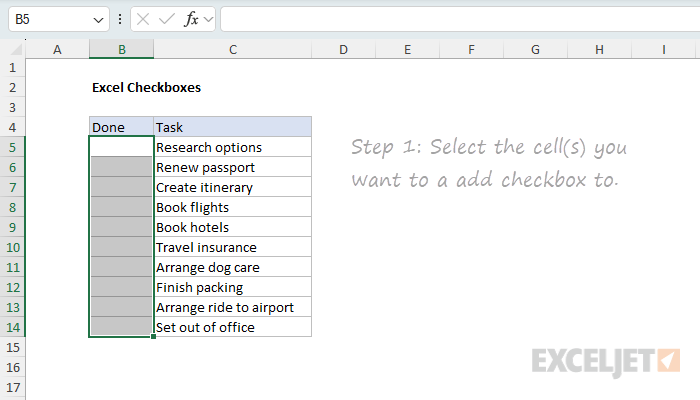
Adding a native checkbox in Excel is easy. First, select the cell(s) you want to add the checkbox to:
Next, click the Checkbox button on the Insert tab of the ribbon:
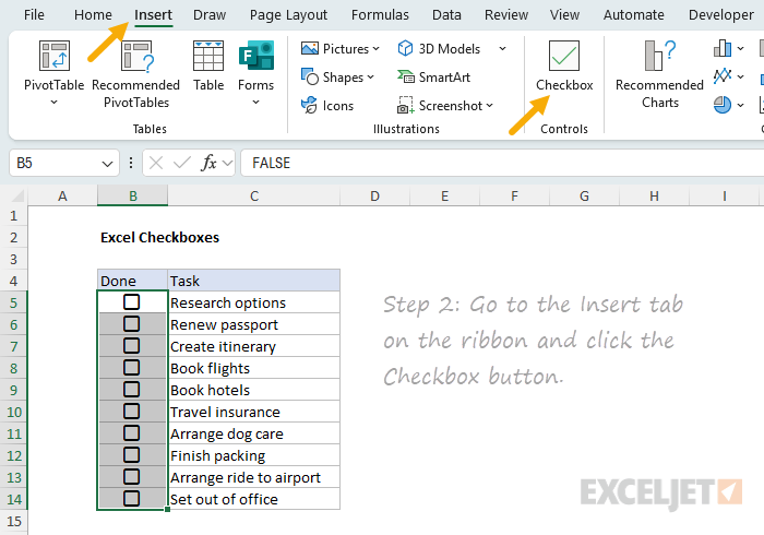
That’s it! You’ve added an interactive checkbox to your cell. You can now click the checkbox to toggle between checked and unchecked as you like:
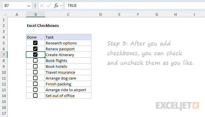
Notice the checkbox will show TRUE (checked) or FALSE (unchecked) in the formula bar as you interact with it.
How to remove a checkbox
The process to remove a checkbox is also very easy. First, select the cells you want to remove the checkbox from:
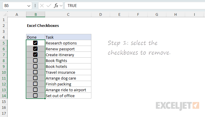
Next, click the Delete key on your keyboard. If a checkbox was checked, it will now be unchecked:
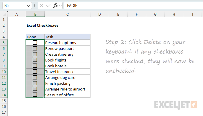
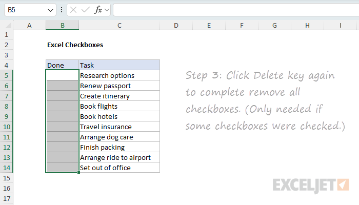
Click the Delete key a second time to completely remove the checkbox:
Checking and unchecking a checkbox
An Excel checkbox is a control that toggles between checked and unchecked. Click once to check it, and click again to uncheck it. If you have more than one checkbox selected, only the first checkbox will be affected.
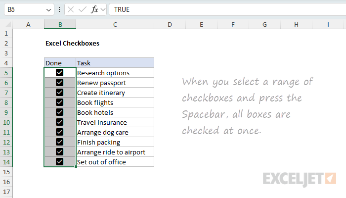
Another way to check and uncheck checkboxes is to use the Spacebar. Press the Spacebar once to check the checkbox, and press it again to uncheck it. A big advantage of the spacebar is that you can use it to check and uncheck all checkboxes in a selection.
First, select the range of checkboxes you want to check or uncheck, then press the Spacebar to check all the checkboxes at once:
If you press the Spacebar again, all the checkboxes will be unchecked:
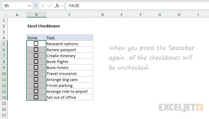
The Spacebar behavior changes if any checkboxes are already checked. If checkboxes in the selection are checked, pressing the Spacebar will uncheck them. Press the Spacebar again to check all checkboxes in the selection.
Example 1: Simple Checklist
A classic use of checkboxes is to create a checklist, useful for tracking the completion of tasks or steps. To create a checklist like this, follow the steps explained above:
- Select the cell(s) you want to add the checkbox to.
- Click the checkbox button on the Insert tab of the ribbon.
- Click the checkbox to toggle between checked and unchecked.
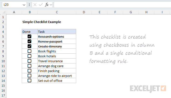
To add a strikethrough effect to the text when the checkbox is checked, use Conditional Formatting. Here are the steps:
- Select the cells you want to format, C5:C14 in this example.
- Navigate to Home > Conditional Formatting > New Rule.
- Select “Use a formula to determine which cells to format” option.
- Enter the formula =$B5 in the formula bar.
- Click the Format button and check the “Strikethrough” option.
- Click OK to save and apply the strikethrough effect.
The screenshot below shows how the rule is configured after adding the formula and setting the strikethrough formatting:
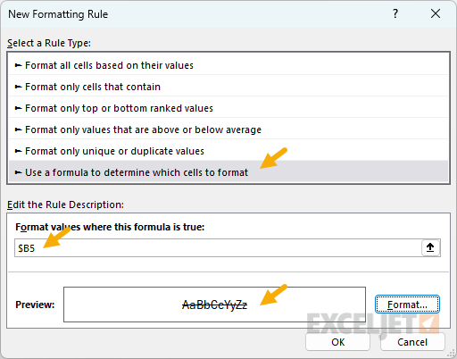
Note: Because checkboxes return TRUE and FALSE, the formula in the conditional formatting rule is simply =$B5 . If you prefer, you can use =$B5=TRUE instead. Also, it’s not strictly necessary to lock the column reference, but it’s useful when you want to copy the rule to other columns.
If you are new to the concept of applying a conditional formatting rule with a formula, watch this short video: How to apply conditional formatting with a formula .
Example 2: Highlight rows with a checkbox
Another useful way to use checkboxes is to highlight rows of interest, as seen in the worksheet below:
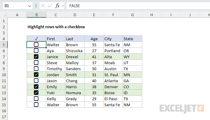
Like the previous example, the formatting is applied using Conditional Formatting. Here are the steps:
- Select the cells you want to format, B5:G15 in this example.
- Navigate to Home > Conditional Formatting > New Rule.
- Select “Use a formula to determine which cells to format” option.
- Enter the formula =$B5 in the formula bar.
- Click the Format button and set a Fill color
- Click OK to save and apply the highlight effect.
The screenshot below shows how the rule is configured after adding the formula and setting the fill color:
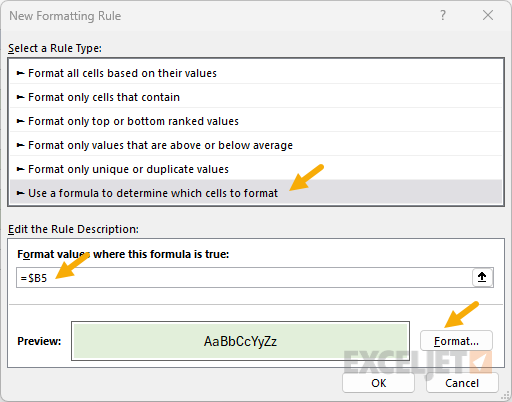
Note: This is a case where we need the mixed reference =$B5 to lock the column and so that it does not change as it is evaluated across all six columns
Example 3: Count and sum checkboxes
Once you are using checkboxes in a worksheet, you may want to count or sum the number of checkboxes that are checked, or sum the values associated with checked or unchecked checkboxes. You can easily do this with the COUNTIFS function and SUMIFS function as shown in the worksheet below:
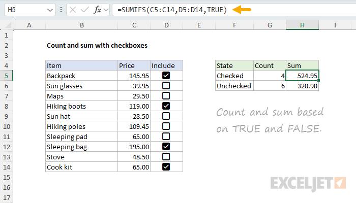
The formulas in column G are set up to count the number of checkboxes that are checked or unchecked D5:D14 using COUNTIFS. The formulas in column H are set up to sum the values in C5:C14 for the checkboxes that are checked or unchecked in D5:D14 using SUMIFS.
G5: =COUNTIFS(D5:D14,TRUE)
G6: =COUNTIFS(D5:D14,FALSE)
H5: =SUMIFS(C5:C14,D5:D14,TRUE)
H6: =SUMIFS(C5:C14,D5:D14,FALSE)
Note that for criteria, we simply use TRUE or FALSE, which is the result of the checkbox.
Example 4: Change formula output with a checkbox
Because checkboxes return TRUE or FALSE, you can use them to change the output of a formula. For example, you can use the result from a checkbox with the IF function to apply a discount or penalty to a value based on whether the checkbox is checked or unchecked. You can see an example of this in the worksheet below, where a checkbox in column D is used to apply a 20% discount to the Price in column C:
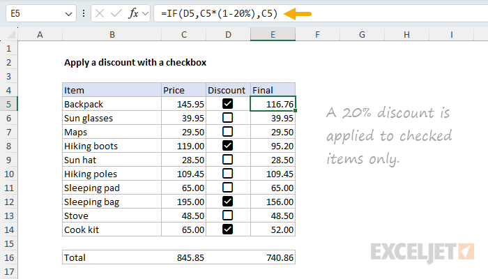
The formula in column E looks like this:
=IF(D5,C5*(1-20%),C5)
Inside the IF function , the logical test is D5 , which is the result of the checkbox. If the checkbox is checked, the formula returns C5*(1-20%) , which is the price minus 20%. If the checkbox is unchecked, the formula returns C5 , which is the original price.
Note: Applying a discount is just one example of how you can use checkboxes to change the output of a formula. Because checkboxes return TRUE or FALSE, you can use them to change the output of almost any formula.
Example 5: Filter a list with a checkbox
Another useful way to use checkboxes is to filter a list based on the checkbox status. You can see an example of this in the worksheet below, where a checkbox in column B (RSVP) is used to filter names in column C with the FILTER function :
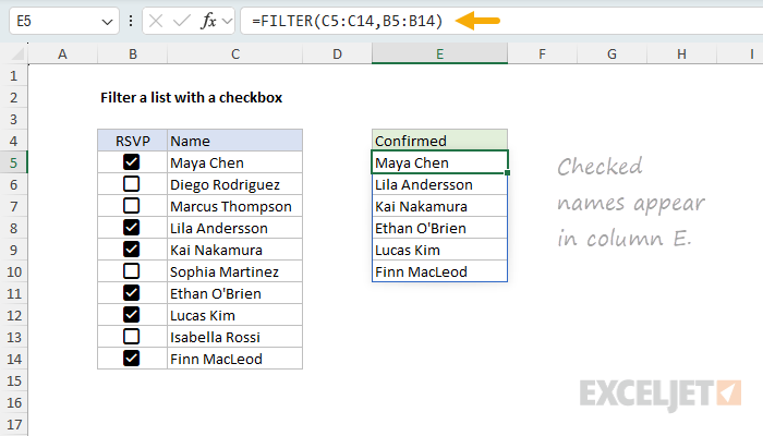
The idea is to create a list of names that have RSVP’d “Yes” to an event. The formula in cell E5 looks like this:
=FILTER(C5:C14,B5:B14)
Inside the FILTER function , the array is given as C5:C14 , which is the range of names to filter. The include argument is B5:B14 , which is the range of checkboxes to filter by. Because checkboxes return TRUE or FALSE, the result from FILTER is a list of names in column C where RSVP is TRUE (checked).
Other important information
Here are a few other things you should know about using new native checkboxes in Excel:
- Checkboxes are a little like number formatting in that you can copy and paste checkbox formatting using Paste Special > Formats on top of TRUE and FALSE values, and the checkboxes will display correctly. However, if you select a checkbox and examine the Checkbox button on the Insert tab of the ribbon, there is no indication that checkbox formatting has been “applied”.
- One difference between checkboxes and number formatting is that inserting checkboxes adds actual values to cells in the worksheet. By default, all checkboxes are unchecked, and the value is FALSE. As you tick off checkboxes, the values change to TRUE. If you remove the checkboxes from cells, the TRUE and FALSE values are also removed.
- If you want to turn off the display of checkboxes but keep the TRUE and FALSE values intact, first select the checkboxes, then navigate to Home > Clear > Clear Formats. You can also put a zero in another cell, copy the zero, then select the checkboxes and use Paste Special > Add to convert the checkboxes to TRUE and FALSE values.
- If you have existing formulas that return TRUE and FALSE, and you insert checkboxes on top of these formulas, the checkboxes will appear correctly. However, checkboxes applied to formulas are read-only; you can’t change the state by clicking. The formula underneath the checkbox is the only mechanism that will check and uncheck the box.
