Explanation
In this example, the goal is to return the most frequently occurring text based on one or more supplied criteria. Working from the inside out, we use the MATCH function to match the text range against itself, by giving MATCH the same range for lookup value and lookup array, with zero for match type:
MATCH(supplier,supplier,0)
Since the lookup value is an array with 10 values, MATCH returns an array of 10 results:
{1;1;3;3;5;1;7;3;1;5;5}
Each item in this array represents the first position at which a supplier name appears in the data. This array is fed into the IF function , which is used to filter results for Client A only:
IF(client=F5,{1;1;3;3;5;1;7;3;1;5;5})
IF returns the filtered array to the MODE function :
{1;FALSE;3;FALSE;5;1;FALSE;FALSE;1;5;FALSE}
Notice only positions associated with Client A remain in the array. MODE ignores FALSE values and returns the most frequently occurring number to the INDEX function as the row number:
=INDEX(supplier,1)
Finally, with the named range “supplier” as the array, INDEX returns “Brown”, the most frequently occurring supplier for Client A.
Mode of text from every other row
Following the example above, the formula below has been adapted to return the most frequent text from every other row. The formulas in E5 and E6 are:
=INDEX(text,MODE(IF(MOD(ROW(text),2)=1,MATCH(text,text,0)))) // odd
=INDEX(text,MODE(IF(MOD(ROW(text),2)=0,MATCH(text,text,0)))) // even
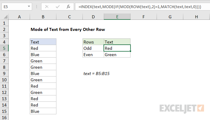
The overall structure of the formulas above is the same as the original example above. The key difference is the logical test used to check even and odd rows with the named range text (B5:B15). Both formulas use the MOD function with a divisor of 2:
MOD(ROW(text),2)=1 // check for odd
MOD(ROW(text),2)=0 // check for even
If the remainder is 1, we have an odd row. If the remainder is 0 (zero), we have an even row. These tests act as a filter for incoming text so that the result from the first formula is the most frequently occurring text in odd rows, and the result from the second formula is the most frequently occurring text in even rows.
Explanation
Working from the inside out, the MATCH function matches the range against itself. That is, we give the MATCH function the same range for lookup value and lookup array (B5:F5).
Because the lookup value contains more than one value (an array), MATCH returns an array of results, where each number represents a position. In the example shown, the array looks like this:
{1,2,1,2,2}
Wherever “dog” appears, we see 2, and Wherever “cat” appears, we see 1. That’s because the MATCH function always returns the first match, which means subsequent occurrences of a given value will return the same (first) position.
Next, this array is fed into the MODE function. MODE returns the most frequently occurring number, which in this case is 2. The number 2 represents the position at which we’ll find the most frequently occurring value in the range.
Finally, we need to extract the value itself. For this, we use the INDEX function. For array, we use the range of values (B5:F5). The row number is provided by MODE.
INDEX returns the value at position 2, which is “dog”.
Empty cells
To deal with empty cells, you can use the following array formula, which adds an IF statement to test for empty cells:
{=INDEX(B5:F5,MODE(IF(B5:F5<>"",MATCH(B5:F5,B5:F5,0))))}
This is an array formula , and must be entered with control + shift + enter.
