Purpose
Return value
Syntax
=MROUND(number,significance)
- number - The number that should be rounded.
- significance - The multiple to use when rounding.
Using the MROUND function
The MROUND function rounds a number to the nearest given multiple. The multiple to use for rounding is provided as the significance argument. Rounding occurs when the remainder from dividing number by significance is greater than or equal to half the value of significance. If the number is already an exact multiple, no rounding occurs and the original number is returned.
The MROUND function takes two arguments , number and significance . Number is the numeric value to round. The significance argument is the multiple to which number should be rounded. In most cases, significance is provided as a numeric value, but MROUND can also understand time entered as text like “0:15” or “0:30”. Number and significance must have the same sign, otherwise MROUND will return a #NUM! error.
Examples
Below are some examples of MROUND formulas with hardcoded values:
=MROUND(10,3) // returns 9
=MROUND(10,4) // returns 12
=MROUND(119,25) // returns 125
To round a number in A1 to the nearest multiple of 5, you can use MROUND like this:
=MROUND(A1,5) // round to nearest 5
Nearest negative number
To round negative numbers with MROUND, use a negative sign for significance:
=MROUND(-10,-3) // returns -9
=MROUND(-10,-4) // returns -12
=MROUND(-119,-25) // returns -125
Nearest .99
MROUND can be used to round pricing to end with .99. The formula below will round a value in A1 to the nearest 1 dollar, subtract 1 cent, and return a final price like $2.99, $5.99, $49.99, etc.
=MROUND(A1,1) - 0.01 // round to nearest .99
Nearest 15 minutes
MROUND can be used to round time. To round a time in A1 to the nearest 15 minutes, you can use a formula like this:
=MROUND(A1,"0:15") // round to nearest 15 min
Rounding functions in Excel
Excel provides a number of functions for rounding:
- To round normally, use the ROUND function .
- To round to the nearest multiple, use the MROUND function .
- To round down to the nearest specified place , use the ROUNDDOWN function .
- To round down to the nearest specified multiple , use the FLOOR function .
- To round up to the nearest specified place , use the ROUNDUP function .
- To round up to the nearest specified multiple , use the CEILING function .
- To round down and return an integer only, use the INT function .
- To truncate decimal places, use the TRUNC function .
Notes
- If a number is already an exact multiple, no rounding occurs.
- Rounding occurs when the remainder from dividing number by significance is greater than or equal to half the value of significance.
- Number and significance must have the same sign.
- MROUND returns #NUM! if number and significance are not the same sign.
- MROUND returns #VALUE! if number or significance is not numeric.
Purpose
Return value
Syntax
=MULTINOMIAL(number1,[number2],...)
- number1 - The first value.
- number2 - [optional] Additional values.
Using the MULTINOMIAL function
The Excel MULTINOMIAL function calculates the multinomial coefficient, which is used to determine the number of ways to assign groups of items into specified sizes. This is especially useful in combinatorics and probability, where you need to count the distinct ways to distribute items into multiple groups, regardless of the order within each group.
Key features
Returns the multinomial coefficient for a set of numbers
Accepts 1 to 255 arguments
All arguments must be non-negative numbers
Returns #VALUE! if any argument is non-numeric
Returns #NUM! if any argument is negative
Key features
Example #1 - Basic usage
Example #2 - Drawing marbles from a bag
Example #3 - Count possible combinations
Example #4 - Calculate probability
Example #5 - Errors
When to use
Formula
Example #1 - Basic usage
The formula below calculates the multinomial coefficient for the numbers 3, 6, and 1:
=MULTINOMIAL(3, 6, 1) // returns 840
This is equivalent to:
=FACT(3+6+1)/(FACT(3)*FACT(6)*FACT(1))
Example #2 - Drawing marbles from a bag
Suppose you have a bag containing 2 red marbles and 2 blue marbles. You draw all 4 marbles one by one and place them in order. We can use the MULTINOMIAL function to count the number of different sequences of colors that could be drawn.
=MULTINOMIAL(2, 2) // returns 6
This counts the number of different color sequences possible when drawing 2 red and 2 blue marbles. The 6 possible sequences are:
- Red, Red, Blue, Blue
- Red, Blue, Red, Blue
- Red, Blue, Blue, Red
- Blue, Red, Red, Blue
- Blue, Red, Blue, Red
- Blue, Blue, Red, Red
Example #3 - Count possible combinations
The MULTINOMIAL function is useful when you have more than two groups and want to count the number of distinct ways to distribute items into groups of specific sizes.
For example, suppose you survey 9 people about their favorite ice cream flavor, and the choices are either chocolate, vanilla, or strawberry. “How many different ways could 2 people pick chocolate, 3 pick vanilla, and 4 pick strawberry?”
We can use the MULTINOMIAL function to count the number of distinct ways to distribute the 9 people into groups of 2, 3, and 4. The formula is:
=MULTINOMIAL(2, 3, 4) // returns 1260
Example #4 - Calculate probability
The MULTINOMIAL function can also be used to calculate probabilities in multinomial distributions. Excel does not provide a dedicated function for the multinomial distribution, so we need to construct the formula manually.
Continuing from the previous example, suppose the probability that a person chooses chocolate is 0.5, vanilla is 0.35, and strawberry is 0.15. Suppose you want to know: “If you survey 9 people, what is the probability that 2 choose chocolate, 3 choose vanilla, and 4 choose strawberry?”
To start, let’s calculate the probability of just one specific way to assign people to flavors: for example, the first two people pick chocolate, the next three pick vanilla, and the last four pick strawberry:
=(0.5^2) * (0.35^3) * (0.15^4) // 7.75195E-06
This value is quite small, because it only accounts for one possible way the outcome could occur. In reality, there are 1260 different ways to assign 2, 3, and 4 people to the three flavors, and each assignment is equally likely. We need to count all possible assignments using the MULTINOMIAL function, and then multiply by the probability of each outcome.
=MULTINOMIAL(2,3,4) * (0.5^2) * (0.35^3) * (0.15^4) // 0.006837223
This gives us the probability that, for our survey of 9 people, 2 choose chocolate, 3 choose vanilla, and 4 choose strawberry.
Example #5 - Errors
All arguments for the MULTINOMIAL function must be numeric and non-negative. If any argument is negative, the function returns #NUM! error.
=MULTINOMIAL(-3, 6, 1) // returns #NUM!
If any argument is non-numeric, the function returns #VALUE! error.
=MULTINOMIAL(3, "a", 1) // returns #VALUE!
When to use
Excel offers several functions for combinatorics and probability. For example, COMBIN and PERMUT can be used for specific types of counting problems involving two groups.
- COMBIN is used for counting combinations of items where order does not matter.
- PERMUT is used for counting permutations of items where order does matter.
The MULTINOMIAL function is more general and is used when you have more than two groups and want to count the number of distinct ways to distribute items into groups of specific sizes, when the order within each group does not matter.
The multinomial coefficient is closely related to the multinomial distribution, which describes the probabilities of counts for more than two possible outcomes (generalizing the binomial distribution). However, Excel does not provide a dedicated function for the multinomial distribution. If you need to calculate multinomial probabilities, you will need to construct the formula manually using the MULTINOMIAL function together with probability terms.
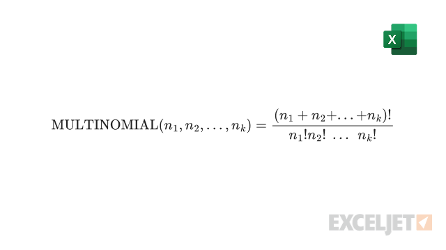
Formula
The MULTINOMIAL function calculates the multinomial coefficient, which is the ratio of the factorial of the sum of the arguments to the product of the factorials of each argument. The formula is: