One of the big changes to Excel in the last year was the introduction of a native checkbox in Excel. Checkboxes might seem like a small thing, but they’re very useful for organizing information, tracking progress, and creating interactive spreadsheets. There’s something uniquely satisfying about ticking a box to finish off a task!
Unlike the clunky solutions of the past, this new checkbox sits happily in a cell and is very easy to set up. Because the checkbox lives in the grid, it will move around naturally as columns and rows are adjusted. Because it returns TRUE or FALSE, you can use the output directly in formulas or to apply conditional formatting. The possibilities are endless.
This article introduces the new native checkbox feature in Excel and walks through a number of practical examples. The examples are in the attached workbook, so download the workbook, follow along, and try the checkboxes out yourself.
For now, native checkboxes are only available in Excel 365. This guide only covers the new native checkbox feature. In older versions of Excel, the process for adding a checkbox is different and more complicated.
- The old days: before native checkboxes
- Key features of native checkboxes in Excel
- How to add a checkbox
- How to remove a checkbox
- Checking and unchecking a checkbox
- Example 1: Simple Checklist
- Example 2: Highlight rows with a checkbox
- Example 3: Count and sum checkboxes
- Example 4: Change formula output with a checkbox
- Example 5: Filter a list with a checkbox
- Other important information
The old days: Before native checkboxes
Until Microsoft added the native, in-cell checkbox in 2024, every “checkbox” in Excel was actually a small shape that floated above the grid. To create a checkbox, you first had to show the Developer tab (hidden by default), choose either a Form-control checkbox or an ActiveX checkbox, drop it onto the sheet, and then link it to a cell so formulas could pick up its TRUE/FALSE value. The boxes didn’t automatically resize or move if you changed row heights or column widths, and they were easy to misalign or delete.
As a result, most people didn’t use checkboxes but instead worked around the problem, using “x” to mark items, showing green ticks with conditional formatting, or creating dropdown lists with “Yes” and “No” options. These solutions work, but they aren’t elegant or intuitive.
The new checkbox lives inside the cell itself, fills down like ordinary data, survives sorting and filtering, and works the same on Windows, Mac, and Excel online. In short, it works like you would expect it to. It’s a real upgrade in usability and a great addition to Excel.
Key features of native checkboxes in Excel
The new native checkbox feature is a useful new addition to your day-to-day work in Excel. It’s easy to use, with a number of useful features:
- A simple way to mark a task as completed.
- One-step process: Ribbon > Insert > Checkbox.
- User-friendly. No need for form controls or developer tools.
- Native in the Excel grid (no floating objects).
- Compatible with Excel formulas and conditional formatting.
- A nice way to make spreadsheets more interactive and intuitive.
- Cross-platform compatibility. Works on Windows, Mac, and Excel online.
How to add a checkbox
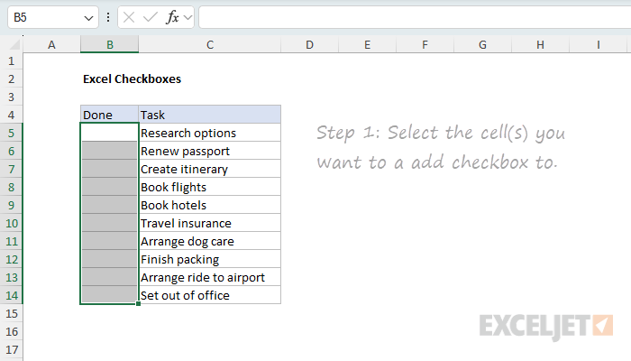
Adding a native checkbox in Excel is easy. First, select the cell(s) you want to add the checkbox to:
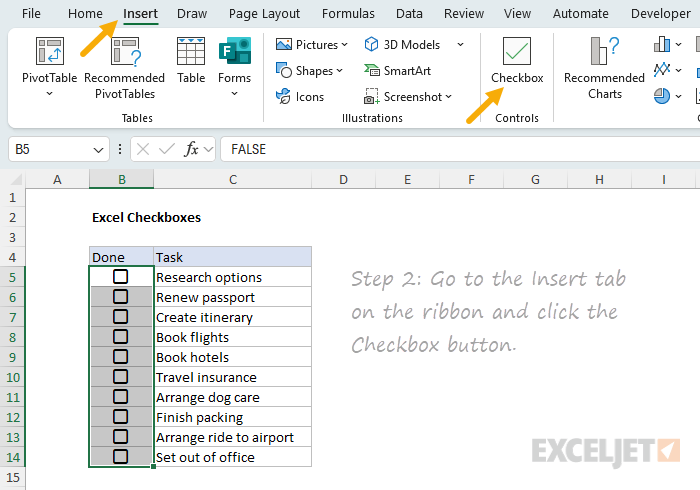
Next, click the Checkbox button on the Insert tab of the ribbon:
That’s it! You’ve added an interactive checkbox to your cell. You can now click the checkbox to toggle between checked and unchecked as you like:
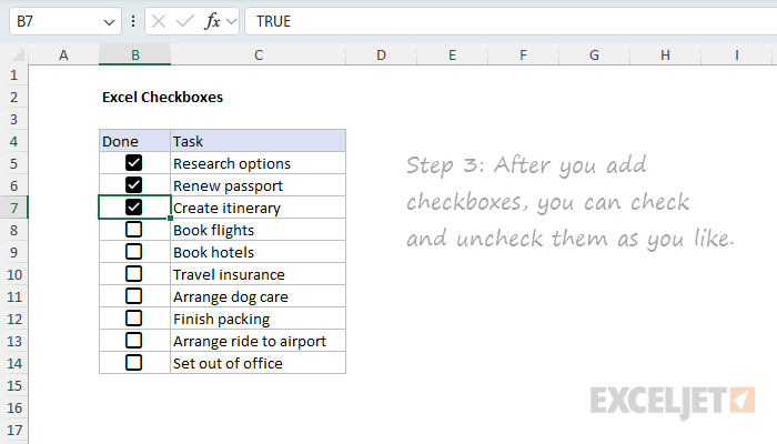
Notice the checkbox will show TRUE (checked) or FALSE (unchecked) in the formula bar as you interact with it.
How to remove a checkbox
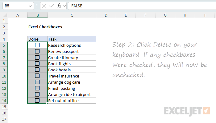
The process to remove a checkbox is also very easy. First, select the cells you want to remove the checkbox from:
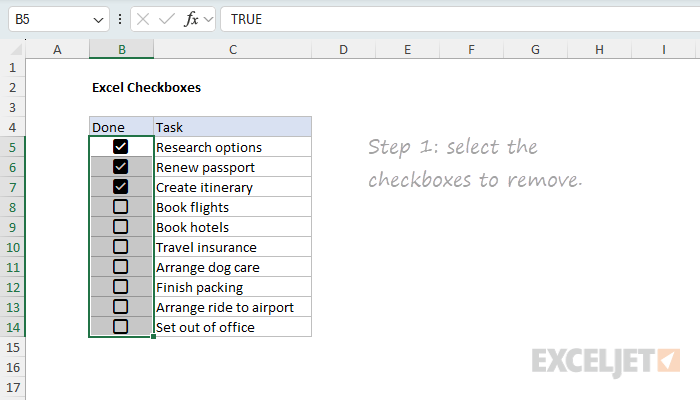
Next, click the Delete key on your keyboard. If a checkbox was checked, it will now be unchecked:
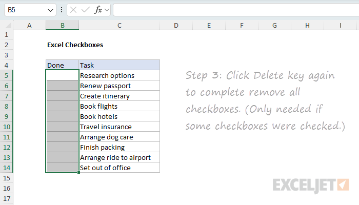
Click the Delete key a second time to completely remove the checkbox:
Checking and unchecking a checkbox
An Excel checkbox is a control that toggles between checked and unchecked. Click once to check it, and click again to uncheck it. If you have more than one checkbox selected, only the first checkbox will be affected.
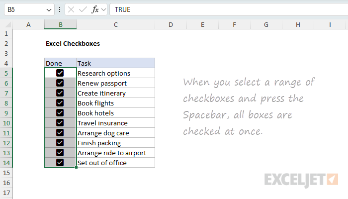
Another way to check and uncheck checkboxes is to use the Spacebar. Press the Spacebar once to check the checkbox, and press it again to uncheck it. A big advantage of the spacebar is that you can use it to check and uncheck all checkboxes in a selection.
First, select the range of checkboxes you want to check or uncheck, then press the Spacebar to check all the checkboxes at once:
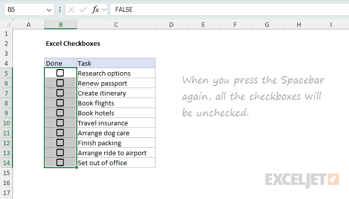
If you press the Spacebar again, all the checkboxes will be unchecked:
The Spacebar behavior changes if any checkboxes are already checked. If checkboxes in the selection are checked, pressing the Spacebar will uncheck them. Press the Spacebar again to check all checkboxes in the selection.
Example 1: Simple Checklist
A classic use of checkboxes is to create a checklist, useful for tracking the completion of tasks or steps. To create a checklist like this, follow the steps explained above:
- Select the cell(s) you want to add the checkbox to.
- Click the checkbox button on the Insert tab of the ribbon.
- Click the checkbox to toggle between checked and unchecked.
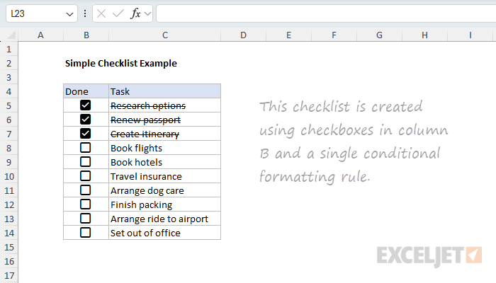
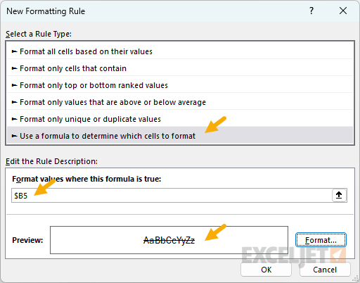
To add a strikethrough effect to the text when the checkbox is checked, use Conditional Formatting. Here are the steps:
- Select the cells you want to format, C5:C14 in this example.
- Navigate to Home > Conditional Formatting > New Rule.
- Select “Use a formula to determine which cells to format” option.
- Enter the formula =$B5 in the formula bar.
- Click the Format button and check the “Strikethrough” option.
- Click OK to save and apply the strikethrough effect.
The screenshot below shows how the rule is configured after adding the formula and setting the strikethrough formatting:
Note: Because checkboxes return TRUE and FALSE, the formula in the conditional formatting rule is simply =$B5 . If you prefer, you can use =$B5=TRUE instead. Also, it’s not strictly necessary to lock the column reference, but it’s useful when you want to copy the rule to other columns.
If you are new to the concept of applying a conditional formatting rule with a formula, watch this short video: How to apply conditional formatting with a formula .
Example 2: Highlight rows with a checkbox
Another useful way to use checkboxes is to highlight rows of interest, as seen in the worksheet below:
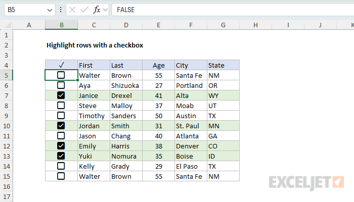
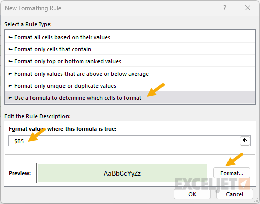
Like the previous example, the formatting is applied using Conditional Formatting. Here are the steps:
- Select the cells you want to format, B5:G15 in this example.
- Navigate to Home > Conditional Formatting > New Rule.
- Select “Use a formula to determine which cells to format” option.
- Enter the formula =$B5 in the formula bar.
- Click the Format button and set a Fill color
- Click OK to save and apply the highlight effect.
The screenshot below shows how the rule is configured after adding the formula and setting the fill color:
Note: This is a case where we need the mixed reference =$B5 to lock the column and so that it does not change as it is evaluated across all six columns
Example 3: Count and sum checkboxes
Once you are using checkboxes in a worksheet, you may want to count or sum the number of checkboxes that are checked, or sum the values associated with checked or unchecked checkboxes. You can easily do this with the COUNTIFS function and SUMIFS function as shown in the worksheet below:
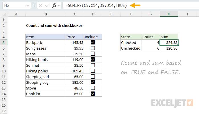
The formulas in column G are set up to count the number of checkboxes that are checked or unchecked D5:D14 using COUNTIFS. The formulas in column H are set up to sum the values in C5:C14 for the checkboxes that are checked or unchecked in D5:D14 using SUMIFS.
G5: =COUNTIFS(D5:D14,TRUE)
G6: =COUNTIFS(D5:D14,FALSE)
H5: =SUMIFS(C5:C14,D5:D14,TRUE)
H6: =SUMIFS(C5:C14,D5:D14,FALSE)
Note that for criteria, we simply use TRUE or FALSE, which is the result of the checkbox.
Example 4: Change formula output with a checkbox
Because checkboxes return TRUE or FALSE, you can use them to change the output of a formula. For example, you can use the result from a checkbox with the IF function to apply a discount or penalty to a value based on whether the checkbox is checked or unchecked. You can see an example of this in the worksheet below, where a checkbox in column D is used to apply a 20% discount to the Price in column C:
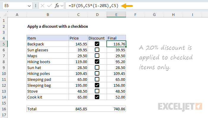
The formula in column E looks like this:
=IF(D5,C5*(1-20%),C5)
Inside the IF function , the logical test is D5 , which is the result of the checkbox. If the checkbox is checked, the formula returns C5*(1-20%) , which is the price minus 20%. If the checkbox is unchecked, the formula returns C5 , which is the original price.
Note: Applying a discount is just one example of how you can use checkboxes to change the output of a formula. Because checkboxes return TRUE or FALSE, you can use them to change the output of almost any formula.
Example 5: Filter a list with a checkbox
Another useful way to use checkboxes is to filter a list based on the checkbox status. You can see an example of this in the worksheet below, where a checkbox in column B (RSVP) is used to filter names in column C with the FILTER function :
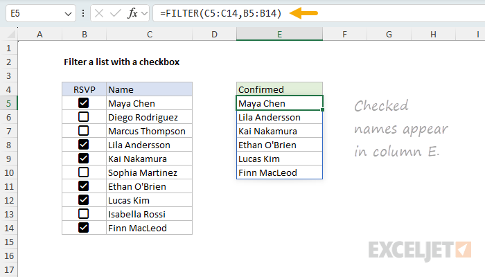
The idea is to create a list of names that have RSVP’d “Yes” to an event. The formula in cell E5 looks like this:
=FILTER(C5:C14,B5:B14)
Inside the FILTER function , the array is given as C5:C14 , which is the range of names to filter. The include argument is B5:B14 , which is the range of checkboxes to filter by. Because checkboxes return TRUE or FALSE, the result from FILTER is a list of names in column C where RSVP is TRUE (checked).
Other important information
Here are a few other things you should know about using new native checkboxes in Excel:
- Checkboxes are a little like number formatting in that you can copy and paste checkbox formatting using Paste Special > Formats on top of TRUE and FALSE values, and the checkboxes will display correctly. However, if you select a checkbox and examine the Checkbox button on the Insert tab of the ribbon, there is no indication that checkbox formatting has been “applied”.
- One difference between checkboxes and number formatting is that inserting checkboxes adds actual values to cells in the worksheet. By default, all checkboxes are unchecked, and the value is FALSE. As you tick off checkboxes, the values change to TRUE. If you remove the checkboxes from cells, the TRUE and FALSE values are also removed.
- If you want to turn off the display of checkboxes but keep the TRUE and FALSE values intact, first select the checkboxes, then navigate to Home > Clear > Clear Formats. You can also put a zero in another cell, copy the zero, then select the checkboxes and use Paste Special > Add to convert the checkboxes to TRUE and FALSE values.
- If you have existing formulas that return TRUE and FALSE, and you insert checkboxes on top of these formulas, the checkboxes will appear correctly. However, checkboxes applied to formulas are read-only; you can’t change the state by clicking. The formula underneath the checkbox is the only mechanism that will check and uncheck the box.
Some older Excel functions don’t spill when you give them a range as input. This article explains why this happens, which functions are affected, and how to fix it.
- Dynamic Arrays and Spilling
- The spilling problem explained
- The simple solution
- List of affected functions
- Why the plus sign?
There are other reasons why a formula might not spill. This article focuses on one specific case: a specific group of older functions that will not accept a range in place of a single value.
Dynamic Arrays and Spilling
In 2019, the Excel team began to introduce dynamic array formulas , a new way to work with data in Excel. In a nutshell, dynamic array formulas can process more than one value at the same time, then return multiple values to the worksheet in a behavior known as " spilling “. Many newer dynamic array functions spill multiple values natively. Good examples are functions like FILTER , SORT , SEQUENCE , and UNIQUE . However, older Excel functions will also spill through a process called " lifting “. When you give a range or array to a function not programmed to accept arrays natively, Excel will “lift” the function and call it multiple times, once for each value in the array. For example, the LEN function is designed to return the number of characters in a text string. If we give LEN the text “apple”, it will return 5:
=LEN("apple") // returns 5
If we give LEN three text strings in an array , it returns an array with three counts, one for each text string:
=LEN({"apple";"banana";"pear"}) // returns {5;6;4}
You can see an example of this in the following worksheet, where the formula in cell D8 looks like this:
=LEN(B8:B10) // returns {5;6;4}
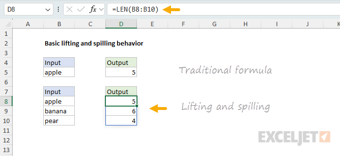
The main thing to understand is that lifting is a built-in behavior that happens automatically. When you give a function more than one value as an input, you will get back multiple results that spill onto the worksheet. It just works. Except when it doesn’t 🙃
The spilling problem explained
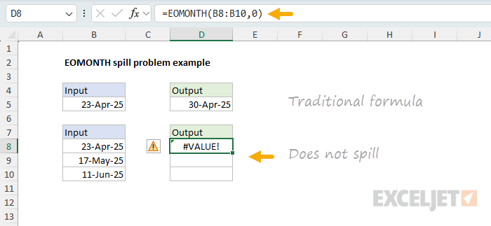
As it turns out, some functions don’t spill when you give them a range instead of a single cell reference. A good example is the EOMONTH function , which returns the last day of the month for any given date. If we give EOMONTH the date 23-Apr-2025, with an offset of 0, it will return the last day of that month, which is 30-Apr-2025. You can see this in the following worksheet, where the formula in cell D5 looks like this:
=EOMONTH(B5,0) // returns 30-Apr-2025
However, if we give EOMONTH a range of three dates, it refuses to spill and instead returns a #VALUE! error with a formula like this in cell D8:
=EOMONTH(B8:B10,0) // returns #VALUE!
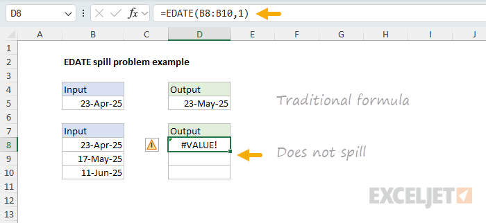
We can see exactly the same problem with the EDATE function , which returns the date a given number of months before or after a given date. If we give EDATE the date 23-Apr-2025, with an offset of 1, it will return the date 23-May-2025. You can see this in the following worksheet, where the formula in cell D5 looks like this:
=EDATE(B5,1) // returns 23-May-2025
However, if we give EDATE a range of three dates, it refuses to spill and instead returns a #VALUE! error with a formula like this in cell D8:
=EDATE(B8:B10,1) // #VALUE! error
What’s going on here? The problem is that some older functions like EOMONTH “resist” spilling when provided a range. This limitation comes from these functions expecting a single cell value instead of a range. The #VALUE! error is essentially reporting the range as an unexpected value. Other common functions that have this same limitation include EDATE, ISEVEN , ISODD , YEARFRAC , WORKDAY , and WORKDAY.INTL . See below for a larger list of affected functions.
The simple solution
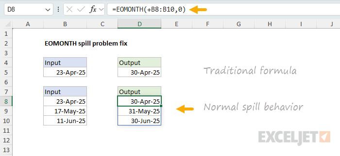
Although this seems like a difficult technical problem, the solution is actually quite simple. The trick is to add a plus sign (+) before the range. This forces Excel to evaluate the range before the function runs. The result is an array of values, which are then passed to the function so that lifting and spilling occur as expected. You can see this fix in the following worksheet, where the formula in cell D8 looks like this:
=EOMONTH(+B8:B10,0) // spills normally
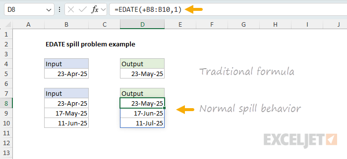
We can do exactly the same thing with the EDATE function, and it will spill normally:
=EDATE(+B8:B10,1) // spills normally
Note: In simple situations like those described above, diagnosing the spill problem and fixing it is fairly straightforward as long as you know about this issue and how to fix it. Where it gets more complicated is when you use a function that resists spilling with a range inside a larger formula. Then, function will return a #VALUE! error that blows up the entire formula, but it will not be so easy to understand what the problem is, since you aren’t actually seeing a function fail to spill on a worksheet.
List of affected functions
The origins of this problem are murky, and it is difficult to find good documentation for Excel functions from the era in which most of these functions were introduced. However, based on conversations with other Excel MVPs, I believe that functions with this spilling limitation all originate from the same development effort: the Analysis ToolPak, which was initially included in Excel 97 as a separate add-in, and later rolled into the core application in Excel 2007. Here is a list of the functions that started life in the Analysis ToolPak:
| Category | Functions |
|---|---|
| Financial | ACCRINT , ACCRINTM , AMORDEGRC , AMORLINC , COUPDAYBS , COUPDAYS , COUPDAYSNC , COUPNCD , COUPNUM , COUPPCD , CUMIPMT * , CUMPRINC , DISC , DOLLARDE , DOLLARFR , DURATION , EFFECT , FVSCHEDULE , INTRATE , MDURATION , NOMINAL , ODDFPRICE , ODDFYIELD , ODDLPRICE , ODDLYIELD , PMT * , PRICE , PRICEDISC , PRICEMAT , RECEIVED , TBILLEQ , TBILLPRICE , TBILLYIELD , XIRR * , XNPV , YIELD , YIELDDISC , YIELDMAT |
| Engineering | BESSELI, BESSELJ, BESSELK, BESSELY, BIN2DEC , BIN2HEX , BIN2OCT , COMPLEX , CONVERT , DEC2BIN , DEC2HEX , DEC2OCT , DELTA , ERF, ERFC, GESTEP, HEX2BIN , HEX2DEC , HEX2OCT , IMABS , IMAGINARY , IMARGUMENT , IMCONJUGATE , IMCOS , IMDIV , IMEXP , IMLN , IMLOG10 , IMLOG2 , IMPOWER , IMPRODUCT * , IMREAL , IMSIN , IMSQRT , IMSUB , IMSUM * , OCT2BIN , OCT2DEC , OCT2HEX |
| Math & Trig | FACTDOUBLE , GCD * , LCM * , MROUND , MULTINOMIAL * , QUOTIENT , RANDBETWEEN , SERIESSUM, SQRTPI |
| Date & Time | EDATE , EOMONTH , NETWORKDAYS , WEEKNUM , WORKDAY , YEARFRAC |
| Information | ISEVEN , ISODD |
| Text | ASC |
Credit: I put together this list using this page on bettersolutions.com .
I quickly tested all of the functions in the list above. Most of them have the spill problem, but there are a few exceptions, which I’ve marked with an asterisk (*) above. Note also that there are a number of functions derived from the ATP functions above that have the spill problem, including WORKDAY.INTL , NETWORKDAYS.INTL , ERF.PRECISE, and ERFC.PRECISE.
When testing these functions, the basic approach is to provide a range in place of any argument that would normally be provided as a single cell reference. For the above functions, the result is usually a #VALUE! error, with exceptions as noted. When you add the plus (+) sign before the range, the formula should lift and spill, and you should get more than one result, depending on the size of the range provided.
Why the plus sign?
Way back in the 1980s, Lotus 1-2-3 was the dominate spreadsheet application, and it allowed you to start a formula with a plus sign (+) instead of an equal sign (=). When Excel added Lotus compatibility in the 1990s, it accepted that syntax, so users migrating to Excel often typed +A1 or +SUM(B2:B10) , which Excel quietly converted to =+A1 and =+SUM(B2:B10) . In Excel, the extra “+” is ignored; it’s just an identity operator. In Excel, the + operator has no effect on a single value, but it will coerce a range into an array , which sidesteps the legacy scalar (i.e., single value) restriction that creates the spilling problem described in this article.
Researching this was interesting. It helped me understand why you occasionally see the + operator turn up in all kinds of simple formulas. I think the reason is that the people who wrote these formulas learned on Lotus 1-2-3. 🙂 I also think it is a matter of convenience for people who use a 10-key (the numeric keypad on a computer keyboard). I ran into many variations of this comment: When I’m typing on the 10 key, I don’t have to move my hand to start a formula with = .. I just hit + with my pinky and start typing. Excel puts the = in on it’s own. We don’t actually type “=+”.
Summary
Excel’s dynamic array formulas were introduced in Excel 365 starting in 2019. A key feature of dynamic arrays is the ability to process multiple values and return multiple results through " spilling .” While newer functions like FILTER and SORT spill natively, older functions use a process called " lifting, " where Excel automatically calls the function multiple times for each value in an array .
However, certain older functions - primarily those originating from Excel’s Analysis ToolPak - resist spilling when given a range as input. Functions like EOMONTH , EDATE , ISEVEN , ISODD , YEARFRAC , WORKDAY , and WORKDAY.INTL will return a #VALUE! error instead of spilling results because they expect single values rather than ranges.
The solution is simple: add a plus sign (+) before the range reference. For example, =EOMONTH(+A1:A5,1) works where =EOMONTH(A1:A5,1) fails. The + operator forces Excel to evaluate the range first, converting it to an array of values that can then be processed through normal lifting and spilling behavior.
This limitation affects dozens of functions across financial, engineering, math, date/time, and information categories - essentially all functions that were originally part of the Analysis ToolPak add-in.
