Purpose
Return value
Syntax
=NORM.DIST(x,mean,standard_dev,cumulative)
- x - The input value x.
- mean - The center of the distribution.
- standard_dev - The standard deviation of the distribution.
- cumulative - A boolean value that determines whether the probability density function or the cumulative distribution function is used.
Using the NORM.DIST function
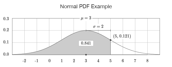
The NORM.DIST function returns values for the normal probability density function (PDF) and the normal cumulative distribution function (CDF). For example, NORM.DIST(5,3,2,TRUE) returns the output 0.841 which corresponds to the area to the left of 5 under the bell-shaped curve described by a mean of 3 and a standard deviation of 2. If the cumulative flag is set to FALSE, as in NORM.DIST(5,3,2,FALSE), the output is 0.121 which corresponds to the point on the curve at 5.
=NORM.DIST(5,3,2,TRUE)=0.841
=NORM.DIST(5,3,2,FALSE)=0.121
The output of the function is visualized by drawing the bell-shaped curve defined by the input to the function. If the cumulative flag is set to TRUE, the return value is equal to the area to the left of the input. If the cumulative flag is set to FALSE, the return value is equal to the value on the curve.
Explanation
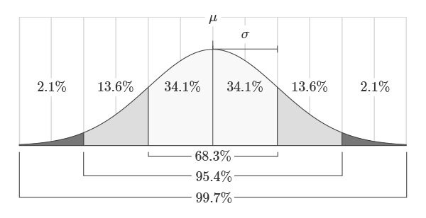
The normal PDF is a bell-shaped probability density function described by two values: the mean and standard deviation. The mean represents the center or “balancing point” of the distribution. The standard deviation represents how spread out the distribution is around the mean. The area under the normal distribution is always equal to 1 and is proportional to the standard deviation as shown in the figure below. For example, 68.3% of the area will always lie within one standard deviation of the mean.
Probability density functions model problems over continuous ranges. The area under the function represents the probability of an event occurring in that range. For example, the probability of a student scoring exactly 93.41% on a test is very unlikely. Instead, it is reasonable to compute the probability of the student scoring between 90% and 95% on the test. Assuming that the test scores are normally distributed, the probability can be calculated using the output of the cumulative distribution function as shown in the formula below.
=NORM.DIST(95,μ,σ,TRUE)-NORM.DIST(90,μ,σ,TRUE)
In this example, if we substitute a mean of 80 in for μ and a standard deviation of 10 in for σ , then the probability of the student scoring between 90 and 95 out of 100 is 9.18%.
=NORM.DIST(95,80,10,TRUE)-NORM.DIST(90,80,10,TRUE)=0.0918
Images courtesy of wumbo.net .
Purpose
Return value
Syntax
=NORM.INV(probability,mean,standard_dev)
- probability - The probability of an event occurring below a threshold.
- mean - The mean of the distribution.
- standard_dev - The standard deviation of the distribution.
Using the NORM.INV function
The NORM.INV function returns the inverse of the normal cumulative distribution. Given the probability of an event occurring below a threshold value, the function returns the threshold value associated with the probability. For example, NORM.INV(0.5, 3, 2) returns 3 since the probability of an event occurring below the mean of the distribution is 0.5. Note, the area under a normal distribution within an interval corresponds to the probability of an event occurring within that interval.
=NORM.INV(0.5,3,2 )// Returns 3
Let’s look at another example using the same normal distribution defined by a mean of 3 and standard deviation of 2.
=NORM.INV(0.84134,3,2)// Returns 5
In this case, the threshold corresponding to the probability of 0.84134 is equal to 5. In other words, the probability of an event occurring below 5 for this normal distribution is equal to 0.8413.
Notes
- The mean describes the center or “balancing point” of the normal distribution.
- The standard deviation describes the shape of the bell-shaped curve.
- Valid probability input to the function is within the range (0,1), excluding 0 and 1.
