Purpose
Return value
Syntax
=OCT2HEX(number,[places])
- number - The octal number you want to convert.
- places - [optional] The number of characters to use in the result. If omitted, uses the minimum number of characters necessary.
Using the OCT2HEX function
The OCT2HEX function is used to convert octal numbers (base 8) to hexadecimal numbers (base 16). This is useful when working with different number systems, especially in engineering and computer science applications.
Key features
- Converts octal numbers to hexadecimal numbers
- Handles both positive and negative octal numbers (using two’s-complement for negatives)
- Returns a hexadecimal number as text
To get the octal representation of a hexadecimal number, use the HEX2OCT function.
- Example #1 - Basic conversion
- Example #2 - Using the places argument
- Example #3 - Negative octal numbers
- Example #4 - Error conditions
Example #1 - Basic conversion
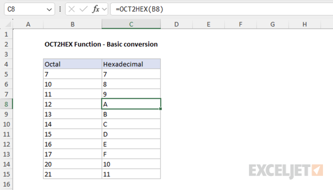
To convert the octal number 12 to hexadecimal, use the following formula:
=OCT2HEX(12) // returns A
The spreadsheet below shows some basic conversions of octal numbers to hexadecimal numbers:
Example #2 - Using the places argument
The places argument in the OCT2HEX function specifies the minimum number of characters to use in the result. When the converted hexadecimal number has fewer characters than the value specified for places , Excel pads the result with leading zeros. This is useful when you want all results to have a consistent length.
For example, to convert the octal number 12 to hexadecimal and pad the result to 3 characters, use:
=OCT2HEX(12, 3) // returns 00A
Places must be a number between 1 and 10, otherwise Excel will return a #NUM! error. If places is not an integer, Excel will truncate the decimal part. If the result is longer than the number specified in places , Excel will return a #NUM! error.
Example #3 - Negative octal numbers
Excel represents negative numbers in non-decimal bases (like octal) using two’s complement notation with a fixed width of 10 characters. This means octal numbers from 0 to 3777777777 represent positive numbers, and octal numbers from 4000000000 to 7777777777 represent negative numbers.
Shown below is a table of the octal numbers from 0 to 7777777777 and their corresponding hexadecimal and decimal numbers:
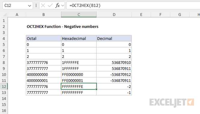
This means the octal numbers from 4000000000 to 7777777777 are mapped to different hexadecimal numbers, because Excel uses two’s complement notation to represent negative numbers. For example, the octal number 4000000000 is mapped to the hexadecimal number FFE0000000 instead of the hexadecimal number 0020000000 .
=OCT2HEX(0377777777, 10) // returns 0003FFFFFF
=OCT2HEX(0400000000, 10) // returns 0004000000
=OCT2HEX(3777777777, 10) // returns 001FFFFFFF
=OCT2HEX(4000000000, 10) // returns FFE0000000
Example #4 - Error conditions
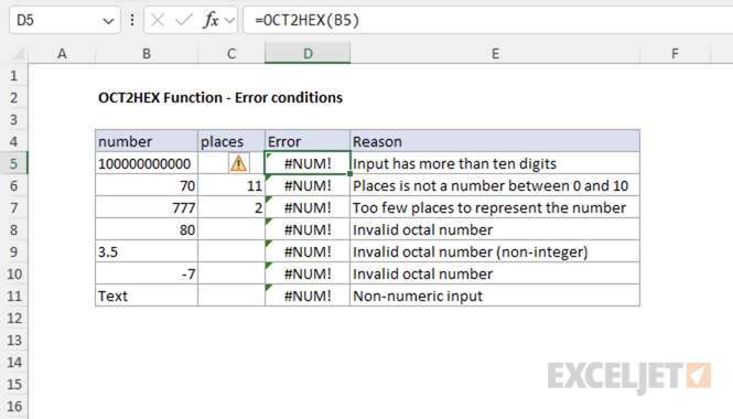
There are several error conditions that can occur when using the OCT2HEX function. For example, if the input contains more than 10 digits, OCT2HEX returns a #NUM! error. This behavior and other error conditions are shown in the example below:
Purpose
Return value
Syntax
=ACCRINT(id,fd,sd,rate,par,freq,[basis],[calc])
- id - Issue date of the security.
- fd - First interest date of security.
- sd - Settlement date of security.
- rate - Interest rate of security.
- par - Par value of security.
- freq - Coupon payments per year (annual = 1, semiannual = 2; quarterly = 4).
- basis - [optional] Day count basis (see below, default =0).
- calc - [optional] Calculation method (see below, default = TRUE).
Using the ACCRINT function
In finance, bonds prices are quoted “clean”. The “clean price” of a bond excludes any interest accrued since the issue date or most recent coupon payment. The “dirty price” of a bond is the price including accrued interest. The ACCRINT function can be used to calculate accrued interest for a security that pays periodic interest, but pay attention to date configuration.
Date configuration
By default, ACCRINT will calculate accrued interest from the issue date. If the settlement date is in the first period, this works. However, if the settlement date is not in the first period, you probably don’t want total accrued interest from the issue date but rather accrued interest from the last interest date (previous coupon date). As a workaround, based on the article here :
- set issue date to the previous coupon date
- set first_interest date to the previous coupon date
Note: According to Microsoft documentation, calc_method controls how total accrued interest is calculated when the date of settlement > first_interest . The default is TRUE, which returns the total accrued interest from issue date to settlement date. Setting calculation method to FALSE is supposed to return accrued interest from first_interest to settlement date. However, I was unable to produce this behavior. In the example below, issue date and first_interest date are set to the previous coupon date (as described above).
Example
In the example shown, we want to calculate accrued interest for a bond with a 5% coupon rate. The issue date is 5-Apr-2018, the settlement date is 1-Feb-2019, and the last coupon date is 15-Oct-2018. We want accrued interest from October 15, 2018 to February 1, 2019. The formula in F5 is:
=ACCRINT(C9,C9,C8,C6,C5,C12,C13,TRUE)
With these inputs, the ACCRINT function returns $14.72, with currency number format applied.
Entering dates
In Excel, dates are serial numbers . Generally, the best way to enter valid dates is to use cell references, as shown in the example. To enter valid dates directly inside a function, you can use the DATE function . To illustrate, the formula below has all values hardcoded. The DATE function is used to supply each of the three required dates:
=ACCRINT(DATE(2018,10,15),DATE(2018,10,15),DATE(2019,2,1),0.05,1000,2,0,TRUE)
Basis
The basis argument controls how days are counted. The ACCRINT function allows 5 options (0-4) and defaults to zero, which specifies US 30/360 basis. This article on wikipedia provides a detailed explanation of available conventions.
| Basis | Day count |
|---|---|
| 0 or omitted | US (NASD) 30/360 |
| 1 | Actual/actual |
| 2 | Actual/360 |
| 3 | Actual/365 |
| 4 | European 30/360 |
Notes
- In Excel, dates are serial numbers .
- All dates, plus frequency and basis , are truncated to integers.
- If dates are invalid (i.e. not actually dates) ACCRINT returns #VALUE!
- ACCRINT returns #NUM when: issue date >= settlement date rate < 0 or par <= 0 frequency is not 1, 2, or 4 Basis is out-of-range
