Purpose
Return value
Syntax
=OR(logical1,[logical2],...)
- logical1 - The first condition or logical value to evaluate.
- logical2 - [optional] The second condition or logical value to evaluate.
Using the OR function
The OR function is one of Excel’s logical functions. It is designed to test multiple conditions simultaneously and return TRUE if any condition is TRUE. If all conditions are FALSE, the OR function returns FALSE. The OR function is often combined with other functions like AND, NOT, and IF to construct more complex logical tests. It commonly appears in the logical test of the IF function and in formulas for conditional formatting and data validation. The OR function is a good way to simplify complicated formulas use many nested IFs .
OR function basics
The purpose of the OR function is to evaluate more than one logical test at the same time and return TRUE if any result is TRUE . Excel’s OR function can handle up to 255 separate conditions, which are entered as arguments with names like “logical1”, “logical2”, and “logical3”, etc. Each “logical” is a condition that can be evaluated as TRUE or FALSE. The arguments provided to the OR function can be constants, cell references, or logical expressions. OR will return TRUE if any condition is TRUE:
=OR(FALSE,FALSE,TRUE) // returns TRUE
If all conditions are FALSE, OR will return FALSE:
=OR(FALSE,FALSE,FALSE) // returns FALSE
Typically, logical arguments are provided to OR as logical expressions, for example:
=OR(A1>0,A1<5)
=OR(A1>0,B1>0)
=OR(A1="red",B1="small")
All expressions in the formulas above will be evaluated as TRUE or FALSE. Notice that text values used in comparisons must be enclosed in double quotes (""). Be aware that OR will also evaluate numbers as TRUE or FALSE, and treat any number except zero (0) as TRUE . You can see this behavior in the formulas below:
=OR(0,0,3) // returns TRUE
=OR(0,0,0) // returns FALSE
Let’s look at some practical ways to use the OR function.
Example - value is x or y or z
You can use OR to test for one of several values. For example, in the worksheet below, we are using the OR function to test if the codes in column B are 115, 120, or 125. The formula in cell D5 is:
=OR(B5=115,B5=120,B5=125)
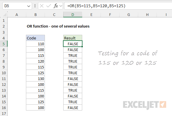
Notice that we are testing for numeric values so the numbers appear in their raw form without quotes ("").
Example - OR with the IF function
The OR function is often embedded inside the IF function as the logical test to simplify what would otherwise be a more complex formula. For example, in the worksheet below, the goal is to test scores in columns B and C. If either score is below 750, the result should be “Deny”. If both scores are 750 or above, the result should be “Approve”. The formula in cell E5 is:
=IF(OR(B5<750,C5<750),"Deny","Approve")
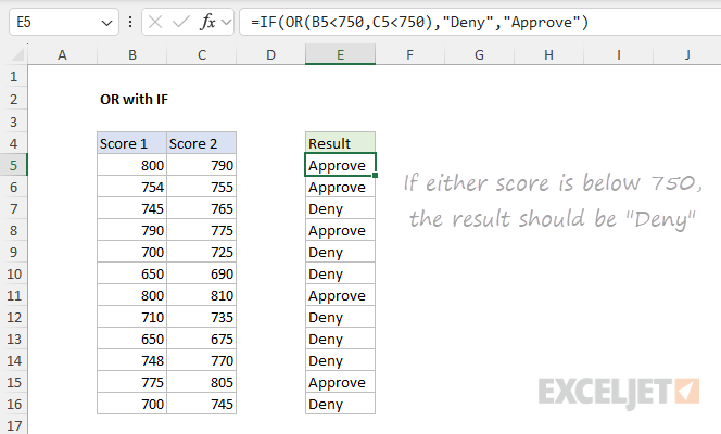
As the formula is copied down, it returns “Approve” or “Deny” for each row in the data.
Example - IF this OR that
The worksheet below is a variation of the example above. This time, the goal is to flag rows where the color is “red” and the size is “small”. The formula in cell D5 is:
=IF(OR(B5="red",B5="green"),"x","")
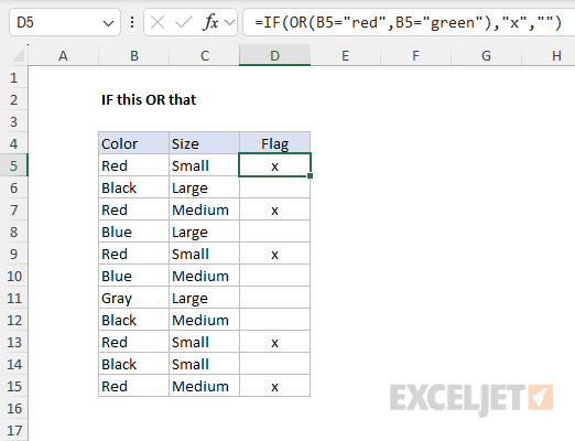
You are free to replace “x” with any other value. Notice that the OR function is not case-sensitive . The lowercase “red” and “small” text strings equal the “Red” and “Small” text on the worksheet.
Example - OR with AND
You can combine the OR function with the AND function to build more advanced conditions. In the worksheet below, the goal is to identify records where the color is “red” or “green” and the quantity is over 100. The logical test inside the IF function is created with AND and OR:
AND(OR(B5="red",B5="green"),C5>100)
The complete formula in E5 is:
=IF(AND(OR(B5="red",B5="green"),C5>100),"x","")
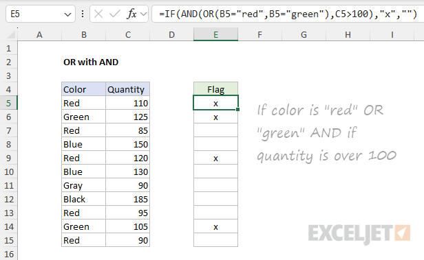
Notice that the text values “red” and “green” are enclosed in double quotes ("") but the number 100 is not .
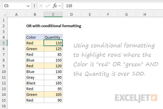
Example - OR with conditional formatting
The OR function is often used in the rules that trigger conditional formatting. In the worksheet below, we have adapted the formula in the example above to apply conditional formatting to rows where the color is “red” or “green” and the quantity is over 100. The conditional formatting is applied to the range B5:C15, and the formula to trigger the rule looks like this:
=AND(OR($B5="red",$B5="green"),$C5>100)
Notice $B5 and $C5 are mixed references with the column fixed in order to highlight entire rows.
Example - OR with a range
It is possible to use OR with a range of values. In the worksheet below, the formula in cell J5 is:
=IF(OR(C5:H5<65),"Fail","Pass")
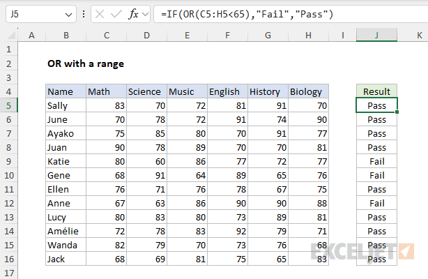
Note: this is an array formula and must be entered with Control + Shift + Enter in Excel 2019 and earlier. In Excel 2021 or later, the formula “just works” without special handling.
Pro-tip - as seen above, the OR function will aggregate multiple results into a single result. This means OR can’t be used in array operations that must create an array of results. To work around this limitation, you can use Boolean logic . For more information, see Array formulas with AND and OR logic .
Notes
- Each logical condition must evaluate to TRUE or FALSE.
- Text values or empty cells supplied as arguments are ignored.
- The OR function will return #VALUE if no logical values are found
- The OR function can handle up to 255 conditions in Excel.
- If any condition is TRUE, OR returns TRUE
- If all conditions are FALSE, OR returns FALSE
- The OR function is not case-sensitive.
- The OR function does not support wildcards .
Purpose
Return value
Syntax
=SWITCH(expression,val1/result1,[val2/result2],...,[default])
- expression - The value or expression to match against.
- val1/result1 - The first value and result pair.
- val2/result2 - [optional] The second value and result pair.
- default - [optional] The default value to use when no match is found.
Using the SWITCH function
The SWITCH function compares one value against a list of values and returns a result that corresponds to the first match found. You can use the SWITCH function when you want to perform a “self-contained” exact match lookup with several possible results. When no match is found, SWITCH can return an optional default value.
The first argument in SWITCH is called “expression” and can be a hard-coded constant, a cell reference, or a formula that returns a specific value to match against. Matching values and corresponding results are entered in pairs. SWITCH can handle up to 126 pairs of values and results. The last argument, default , is an optional value to return when there is no match.
In the example shown, the formula in D5 is:
=SWITCH(C5,1,"Poor",2,"OK",3,"Good","?")
SWITCH only performs an exact match, so you can’t include logical operators like greater than (>) or less than (<) in the logic used to determine a match. You can work around this limitation by constructing a formula to match against TRUE like this:
=SWITCH(TRUE,A1>=1000,"Gold",A1>=500,"Silver","Bronze")
However, in a case like this, the IFS function would likely be more straightforward.
SWITCH and performance
You might expect SWITCH to stop evaluating once it finds a matching value, but in fact, Excel evaluates every expression in the formula , even for cases that are not used. This can degrade performance when any expressions involve complex or time-consuming calculations.
In recursive LAMBDA functions, this behavior can also cause problems because unused result branches are still evaluated, potentially causing unwanted recursion and a #NUM error.
If you need “short-circuit” behavior, where Excel stops evaluating after finding the first match, consider using nested IF functions instead. The IF function performs true short-circuit evaluation, skipping unnecessary calculations once a match is found.
SWITCH versus IFS
Like the IFS function , the SWITCH function allows you to test more than one condition without nesting multiple IF statements in a single self-contained formula. SWITCH therefore makes it easier to write (and read) a formula with many conditions. One advantage of SWITCH over IFS is that the expression appears just once in the function and does not need to be repeated. However, SWITCH is limited to exact matching. It is not possible to use operators like greater than (>) or less than (<) with the standard syntax. In contrast, the IFS function actually requires expressions for each condition, so you can use logical operators as needed.
Notes
- Expression can be another formula that returns a specific value.
- SWITCH can handle up to 126 value/result pairs.
- Enter a final argument to set a default result when no match is found.
- SWITCH does not have short-circuit behavior; all expressions are evaluated
