The “Percentage” number format is one of the built-in number formats in Excel. In mathematics, a percentage is a number expressed as a fraction of 100. The word percent literally means “per one-hundred”. For example, 65% is read as “Sixty-five percent” and is equivalent to 65/100 or 0.65.
To apply the percentage number format to a number, first select the number(s), then use any of these methods:
- Use the keyboard shortcut Control + Shift + Enter
- Select “Percentage” from the dropdown on the home tab of the ribbon
- Click the % button in the Number section on the home tab of the ribbon
- Control + 1 > Number > Percentage
Applying percentage format does not change the number, only the display of the number. In the screen above, the numbers in column B are the same as the numbers in column D.
By default, Excel will display the number with the percent sign (%) and no decimal places. To adjust this format, open the Format Cells dialog box, select Percentage, then select Custom. There you can adjust the codes in the “Type” input area. For example:
0% // default, zero decimals
0.00% // two decimal places
For more information on custom number format codes see: Custom Number Formats .
A Pivot Table is a special tool in Excel for summarizing data without formulas. The Pivot Table interface behaves like a report generator, allowing you to interactively add and remove fields as you like. The screen below shows the how fields have been configured to build the pivot table shown above.
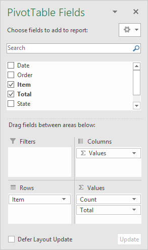
When data changes, you can simply refresh the pivot table to see a new summary. Pivot tables automatically group data using field values.
For more details and examples, see Excel Pivot Tables .
