Purpose
Return value
Syntax
=PERCENTILE.INC(array,k)
- array - Data values.
- k - Number representing kth percentile.
Using the PERCENTILE.INC function
The Excel PERCENTILE.INC function calculates the “kth percentile” for a set of data, where k is between 0 and 1, inclusive. A percentile is a value below which a given percentage of values in a data set fall. A percentile calculated with .4 as k means 40% percent of values are less than or equal to the calculated result, a percentile calculated with k = .9 means 90% percent of values are less than or equal to the calculated result.
To use PERCENTILE.INC, provide a range of values and a number between 0 and 1 for the " k " argument, which represents percent. For example:
=PERCENTILE.INC(range,.4) // 40th percentile
=PERCENTILE.INC(range,.9) // 90th percentile
You can also specify k as a percent using the % character:
=PERCENTILE.INC(range,80%) // 80th percentile
PERCENTILE.INC returns a value greater than or equal to the specified percentile.
In the example shown, the formula in G5 is:
=PERCENTILE.INC(scores,E5)
where “scores” is the named range C5:C14.
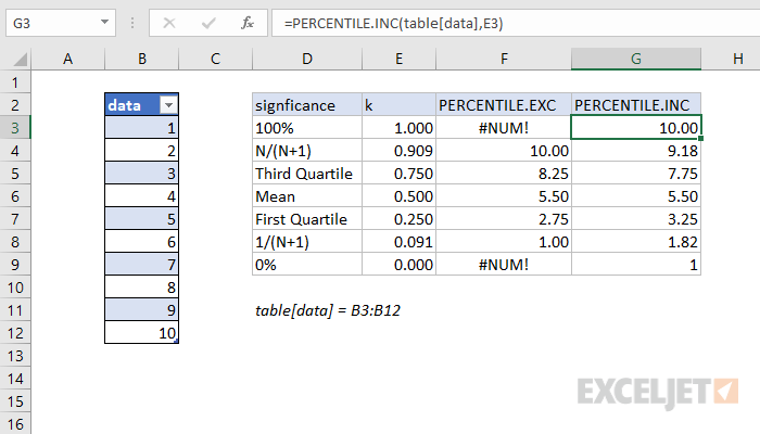
PERCENTILE.INC vs. PERCENTILE.EXC
PERCENTILE.INC includes the full range of 0 to 1 as valid k values, compared to PERCENTILE.EXC which excludes percentages below 1/(N+1) and above N/(N+1).
Note: Microsoft classifies PERCENTILE as a " compatibility function “, now replaced by the PERCENTILE.INC function.
Notes
- k can be provided as a decimal (.5) or a percentage (50%)
- k must be between 0 and 1, otherwise PERCENTILE.INC will return the #NUM! error.
- When percentiles fall between values, PERCENTILE.INC will interpolate and return an intermediate value.
Purpose
Return value
Syntax
=PERCENTRANK(array,x,[significance])
- array - Array of data values.
- x - Value to rank.
- significance - [optional] Number of significant digits in result. Defaults to 3.
Using the PERCENTRANK function
The PERCENTRANK function returns the relative standing of a value within a data set as a percentage. For example, a test score greater than 80% of all test scores is said to be at the 80th percentile. In this case, PERCENTRANK will assign a rank of .80 to the score. To use PERCENTRANK, provide an array of values (typically a range) and the value to rank, x . In the example shown, the formula in C5 is:
=PERCENTRANK(data,B5)
where data is the named range B5:B12. As the formula is copied down, it returns the rank of each value in column B as a decimal value. To display the results in column C as a percentage, apply the percentage number format . The table in the range F4:G15 is for reference only. It uses the PERCENTILE function in column G to calculate a percentile for each value in column F. A percentile is the value below which a given percentage of observations in a group fall.
The named range data is used for convenience only, since named ranges automatically behave like absolute references . If you prefer, you can use an absolute reference like $B$5:$B$12 instead of a named range.
Note: Microsoft classifies PERCENTRANK as a " compatibility function “, now replaced by the PERCENTRANK.INC function.
Inclusive vs. Exclusive
Starting with Excel 2010, the PERCENTRANK function has been replaced by two functions: PERCENTRANK.INC and PERCENTRANK.EXC . The INC version represents “inclusive” behavior, and the EXC version represents “exclusive” behavior. Both formulas use the same arguments.
- Use the PERCENTRANK.EXC function to determine the percentage rank exclusive of the first and last values in the array.
- Use the PERCENTRANK.INC or PERCENTRANK to find the percentage rank inclusive of the first and last values in the array.
Notes
- If x does not exist in the array, PERCENTRANK interpolates to find the percentage rank.
- When significance is omitted PERCENTRANK returns three significant digits (0.xxx)
