Pivot tables are an easy way to quickly count values in a data set. In the example shown, a pivot table is used to count the names associated with each color.
Fields
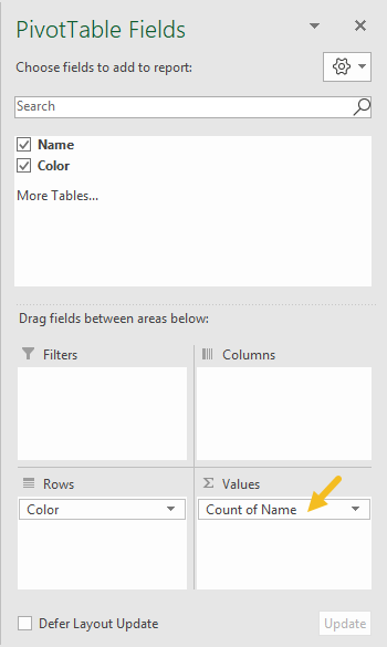
The pivot table shown is based on two fields: Name and Color. The Color field is configured as a row field, and the name field is a value field, as seen below:
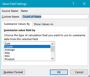
The Name field is configured to summarize by count:
You are free to rename “Count of Name” as you like.
Steps
- Create a pivot table
- Add a category field to the rows area (optional)
- Add field to count to Values area
- Change value field settings to show count if needed
Notes
- Any non-blank field in the data can be used in the Values area to get a count.
- When a text field is added as a Value field, Excel will display a count automatically.
- Without a Row field, the count will be a global count of all data records.
Pivot tables make it easy to quickly sum values in various ways. In the example shown, a pivot table is used to sum amounts by color.
Fields
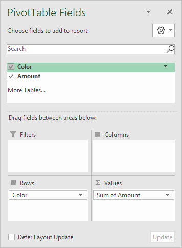
The pivot table shown is based on two fields: Color and Amount . The Color field is configured as a row field, and the Amount field is a value field, as seen below:
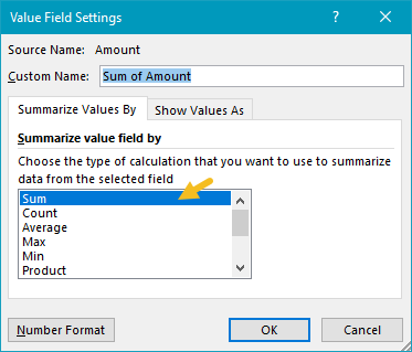
The Amount field is configured to Sum:
You are free to rename “Sum of Name” as you like.
Steps
- Create a pivot table
- Add a category field the rows area (optional)
- Add field to count to Values area
- Change value field settings to show sum if needed
Notes
- When numeric field is added as a Value field, Excel will display a sum automatically.
- Without a Row field, the sum will be the total of all Amounts.
