Pivot tables make it easy to quickly sum values in various ways. In the example shown, a pivot table is used to sum amounts by color.
Fields
The pivot table shown is based on two fields: Color and Amount . The Color field is configured as a row field, and the Amount field is a value field, as seen below:
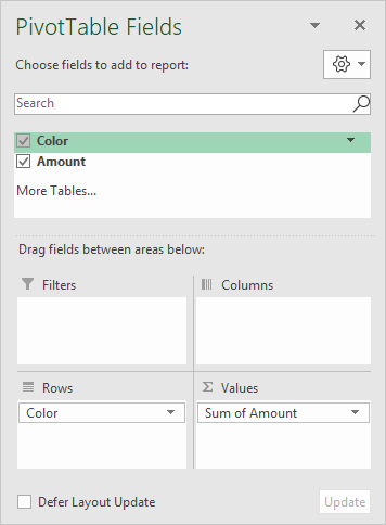
The Amount field is configured to Sum:
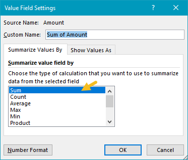
You are free to rename “Sum of Name” as you like.
Steps
- Create a pivot table
- Add a category field the rows area (optional)
- Add field to count to Values area
- Change value field settings to show sum if needed
Notes
- When numeric field is added as a Value field, Excel will display a sum automatically.
- Without a Row field, the sum will be the total of all Amounts.
Standard Pivot Tables have a simple feature for creating calculated fields. You can think of a calculated field as a virtual column in the source data. A calculated field will appear in the field list window, but will not take up space in the source data. In the example shown, a calculated field called “Unit Price” has been created with a formula that divides Sales by Quantity. The pivot table displays the calculated unit price for each product in the source data.
Note: data ends on row 18, so the calculation is as follows: $1,006.75 / 739 = $1.36
Fields
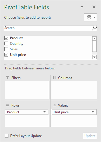
The source data contains three fields, Product, Quantity, and Sales. A fourth field called “Unit Price” is a calculated field.
The calculated field was created by selecting “Insert Calculated Field” in the “Fields, Items, and Sets” menu on the ribbon:
<img loading=“lazy” src=“https://exceljet.net/sites/default/files/images/pivot/inline/pivot%20table%20calculated%20field%20ribbon%20menu.png" onerror=“this.onerror=null;this.src=‘https://blogger.googleusercontent.com/img/a/AVvXsEhe7F7TRXHtjiKvHb5vS7DmnxvpHiDyoYyYvm1nHB3Qp2_w3BnM6A2eq4v7FYxCC9bfZt3a9vIMtAYEKUiaDQbHMg-ViyGmRIj39MLp0bGFfgfYw1Dc9q_H-T0wiTm3l0Uq42dETrN9eC8aGJ9_IORZsxST1AcLR7np1koOfcc7tnHa4S8Mwz_xD9d0=s16000';" alt=“Select “Insert Calculated Field” from this menu - 4”>
The calculated field is named “Unit Price” and defined with the formula “=Sales/Quantity” as seen below:
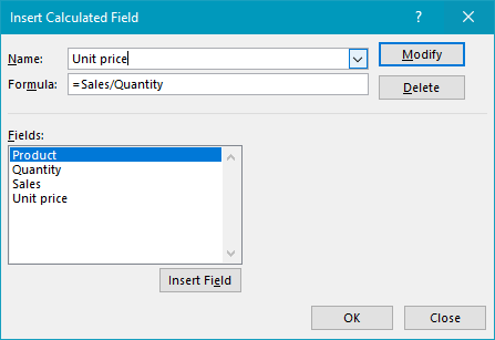
Note: Field names with spaces must be wrapped in single quotes (’). Excel will add these automatically when you click the Insert Field button, or double-click a field in the list.
The Unit Price field is renamed “Unit Price " (note the extra space) after it has been added to the Values area:
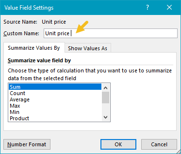
The extra space is required because Excel won’t allow you to use exactly the same field name that appears in the data in a pivot table.
Steps
- Create a pivot table
- Create the Calculated field “Unit Price”
- Add Unit Price to field to Values area Rename field “Unit Price " Set number format as desired
